10: Putting it all together

Overview

You have made it to the last tutorial in the series - congratulations! In this tutorial we will have a look at the reproducibility certification scheme, run some analyses (ANOVAs specifically), and do a bit of data wrangling.

Reproducibility Certification

Since March 2023, the School of Psychology has been running one of the first reproducibility certification schemes for quantitative research in the UK, set up by Prof Zoltan Dienes and Dr Reny Baykova. The scheme operates on a completely voluntary basis and the goal is to help researchers gain the skills to conduct reproducible research.

Anyone who wants to have their results certified as reproducible before submitting their paper for publication needs to share their data, analysis materials, and manuscript with Dr Baykova. She then examines the materials, points out any results that do not reproduce, and provides suggestions on how to improve the reproducibility of the study. After the researchers have updated the materials and manuscript, she completes and uploads a final reproducibility report online.

Researchers can then highlight that their paper has been certified as computationally reproducible and reference the reproducibility report in their manuscript, thus setting them apart in terms of transparency and rigour in the eyes of editors, reviewers, and readers.

Setup

Packages

To set up, there are a lot of packages that we will make our way through today. The key ones are, naturally, {tidyverse}; {afex} for factorial designs; {ggrain} for raincloud plots; {lavaan} for mediation; and {papaja} for pretty formatting and reporting.

Exercise

Load the packages.

Solution

library(tidyverse)
library(afex)
library(ggrain)
library(lavaan)
library(papaja)

Data

Before we get started on the Reproducibility Report, let’s first get some data to work with as we go. Today we’re continuing to work with the dataset courtesy of fantastic Sussex colleague Jenny Terry. This dataset contains real data about statistics and maths anxiety. To save time, for this tutorial, Jennifer has created averaged scores for each overall scale and subscale, and dropped the individual items, so we will not be using the raw data. However, the raw data itself is also available in our project folder on the Cloud, or to download below, if you wish to (later) do the pre-processing from scratch.

Exercise

Read in the dataset and save it in a new object, anx_data.

On the Cloud, you can read in this dataset from the data folder using here::here().

Elsewhere, you can download the dataset, or copy the dataset URL, from the Data and Workbooks page.

Solution

Read in from file:

anx_data <- readr::read_csv(here::here("data/anx_scores_data.csv"))

Read in from URL:

anx_data <- readr::read_csv("https://raw.githubusercontent.com/drmankin/practicum/master/data/anx_scores_data.csv")

You are welcome to instead use another dataset that you are familiar with or are keen to explore. However, remember that anything you upload to Posit Cloud is visible to all workspace admins, so keep GDPR in mind.

There’s quite a bit in the dataset we are using today, but a codebook has already been created, so we are in luck! Refer to the codebook below for a description of all the variables.

Dataset Info Recap

This study explored the difference between maths and statistics anxiety, widely assumed to be different constructs. Participants completed the Statistics Anxiety Rating Scale (STARS) and Maths Anxiety Rating Scale - Revised (R-MARS), as well as modified versions, the STARS-M and R-MARS-S. In the modified versions of the scales, references to statistics and maths were swapped; for example, the STARS item “Studying for an examination in a statistics course” became the STARS-M item “Studying for an examination in a maths course”; and the R-MARS item “Walking into a maths class” because the R-MARS-S item “Walking into a statistics class”.

Participants also completed the State-Trait Inventory for Cognitive and Somatic Anxiety (STICSA). They completed the state anxiety items twice: once before, and once after, answering a set of five MCQ questions. These MCQ questions were either about maths, or about statistics; each participant only saw one of the two MCQ conditions.

Important

For learning purposes, I’ve randomly generated some additional variables to add to the dataset containing info on distribution channel, consent, gender, and age. Especially for the consent variable, don’t worry: all the participants in this dataset did consent to the original study. I’ve simulated and added this variable in later to practice removing participants.

Codebook

Variable	Type	Description	Values
id	Categorical	Unique ID code	NA
distribution	Categorical	Channel through which the study was completed, either as a preview (before real data collection) or anonymous genuine responses. Note that this variable has been randomly generated and does NOT reflect genuine responses.	"preview" or "anonymous"
consent	Categorical	Whether the participant read and consented to participate. Note that this variable has been randomly generated and does NOT reflect genuine responses; all participants in this dataset did originally consent to participate.	"Yes" or "No"
gender	Categorical	Gender identity. Note that this variable has been randomly generated and does NOT reflect genuine responses.	"female", "male", "non-binary", or "other/pnts". "pnts" is an abbreviation for "Prefer not to say".
age	Numeric	Age in years. Note that this variable has been randomly generated and does NOT reflect genuine responses.	18 - 99
mcq	Categorical	Independent variable for MCQ question condition, whether the participant saw MCQ questions about mathematics or statistics.	"maths" or "stats"
stars_test_score	Numeric	Averaged score on the Test Anxiety subscale of the Statistics Anxiety Rating Scale (STARS)	1 (low anxiety) to 5 (high anxiety)
stars_int_score	Numeric	Averaged score on the Interpretation Anxiety subscale of the Statistics Anxiety Rating Scale (STARS)	1 (low anxiety) to 5 (high anxiety)
stars_help_score	Numeric	Averaged score on the Asking for Help subscale of the Statistics Anxiety Rating Scale (STARS)	1 (low anxiety) to 5 (high anxiety)
stars_m_test_score	Numeric	Averaged score on the Test Anxiety subscale of the Statistics Anxiety Rating Scale - Maths (STARS-M), a modified version of the STARS with all references to maths replaced with statistics.	1 (low anxiety) to 5 (high anxiety)
stars_m_int_score	Numeric	Averaged score on the Interpretation Anxiety subscale of the Statistics Anxiety Rating Scale - Maths (STARS-M), a modified version of the STARS with all references to maths replaced with statistics.	1 (low anxiety) to 5 (high anxiety)
stars_m_help_score	Numeric	Averaged score on the Asking for Help subscale of the Statistics Anxiety Rating Scale - Maths (STARS-M), a modified version of the STARS with all references to maths replaced with statistics.	1 (low anxiety) to 5 (high anxiety)
rmars_test_score	Numeric	Averaged score on the Test Anxiety subscale of the Revised Maths Anxiety Rating Scale (R-MARS)	1 (low anxiety) to 5 (high anxiety)
rmars_num_score	Numeric	Averaged score on the Numerical Task Anxiety subscale of the Revised Maths Anxiety Rating Scale (R-MARS)	1 (low anxiety) to 5 (high anxiety)
rmars_course_score	Numeric	Averaged score on the Course Anxiety subscale of the Revised Maths Anxiety Rating Scale (R-MARS)	1 (low anxiety) to 5 (high anxiety)
rmars_s_test_score	Numeric	Averaged score on the Test Anxiety subscale of the Revised Maths Anxiety Rating Scale - Statistics (R-MARS-S), a modified version of the MARS with all references to maths replaced with statistics.	1 (low anxiety) to 5 (high anxiety)
rmars_s_num_score	Numeric	Averaged score on the Numerical Anxiety subscale of the Revised Maths Anxiety Rating Scale - Statistics (R-MARS-S), a modified version of the MARS with all references to maths replaced with statistics.	1 (low anxiety) to 5 (high anxiety)
rmars_s_course_score	Numeric	Averaged score on the Course Anxiety subscale of the Revised Maths Anxiety Rating Scale - Statistics (R-MARS-S), a modified version of the MARS with all references to maths replaced with statistics.	1 (low anxiety) to 5 (high anxiety)
sticsa_trait_score	Numeric	Averaged score on the Trait Anxiety subscale of the State-Trait Inventory for Cognitive and Somatic Anxiety.	1 (not at all) to 4 (very much so)
sticsa_pre_state_score	Numeric	Averaged score on the State Anxiety subscale of the State-Trait Inventory for Cognitive and Somatic Anxiety, pre-MCQ.	1 (not at all) to 4 (very much so)
sticsa_post_state_score	Numeric	Averaged score on the State Anxiety subscale of the State-Trait Inventory for Cognitive and Somatic Anxiety, post-MCQ.	1 (not at all) to 4 (very much so)
mcq_score	Numeric	Total (summed) score on the MCQ questions.	0 (all incorrect) to 5 (all correct)

Reproducibility Report: Part One

The reproducibility report template consists of 8 sections evaluating the reproducibility of different aspects of the study. In the previous tutorials, we largely covered the contents of sections 4 to 8. We will now go through some of the key points in sections 1 to 3 and highlight common pitfalls that jeopardize reproducibility.

Section 1: Reproducibility of Data Processing

This section of the report examines whether the processing of the data prior to conducting statistical analysis is reproducible. Let’s dissect some of the questions in this section.

Question 1

Is the raw data used in the analysis shared publicly? If NO, why not?

Raw data refers to the data exactly as it comes out of the data collection program or software. Ideally, you want to upload the raw data online before you have applied any pre-processing to it. In some cases, the raw data may contain personal identifying information, and therefore needs to be pre-processed to remove any such sensitive information before it is shared online. In this case, the best solution would be to upload the anonymized data online and share the raw data with the person conducting the reproducibility check, so that they can confirm the pre-processing is reproducible and it generates the publicly available data.

RepRoducibility: Never modify raw data

Always keep a backup, untouched copy of your raw data because so many unexpected things can go wrong, such as Excel just changing your data on a whim¹:

Mistaken Identifiers: Gene name errors can be introduced inadvertently when using Excel in bioinformatics (Zeeberg et al, 2004)

Background: When processing microarray data sets, we recently noticed that some gene names were being changed inadvertently to non-gene names.

Results: A little detective work traced the problem to default date format conversions and floating-point format conversions in the very useful Excel program package. The date conversions affect at least 30 gene names; the floating-point conversions affect at least 2,000 if Riken identifiers are included. These conversions are irreversible; the original gene names cannot be recovered.

Conclusions: Users of Excel for analyses involving gene names should be aware of this problem, which can cause genes, including medically important ones, to be lost from view and which has contaminated even carefully curated public databases. We provide work-arounds and scripts for circumventing the problem.

Question 5

Does the shared data include a description of the data?

Making data available online is just the first step of making your study reproducible. The next step is to ensure that other people can use the data you have shared, and to do so, they should be able to navigate the repository and figure out what all the shared materials mean and do, and how they interact with each other. To help other researchers use the materials you have shared as you intended them to be used, online repositories should be accompanied by a description of the structure of the repository (what folder contains what files) and a data dictionary describing any data that is shared.

RepRoducibility: The FAIR Principles of Data Sharing

According to the cleverly named FAIR principles of data sharing, data should be Findable, Accessible, Interoperable, Reusable:

The FAIR Guiding Principles for scientific data management and stewardship (Wilkinson et al. 2016)

There is an urgent need to improve the infrastructure supporting the reuse of scholarly data. A diverse set of stakeholders representing academia, industry, funding agencies, and scholarly publishers have come together to design and jointly endorse a concise and measureable set of principles that we refer to as the FAIR Data Principles. The intent is that these may act as a guideline for those wishing to enhance the reusability of their data holdings. Distinct from peer initiatives that focus on the human scholar, the FAIR Principles put specific emphasis on enhancing the ability of machines to automatically find and use the data, in addition to supporting its reuse by individuals. This Comment is the first formal publication of the FAIR Principles, and includes the rationale behind them, and some exemplar implementations in the community.

I (RB) have found that the main reason people avoid writing readme files and data dictionaries is that they take a lot of time to put together, and the process is genuinely not fun². However, the payoffs are great and more than justify the hour or so of boredom you’d experience. In some cases, preparing these descriptions can even help you figure out if you’ve used the correct data and variables in your analysis code. So, make yourself a cup of hot beverage and go for it. This Cornell guide to writing readme documents is a good place to get you started, and if you have labelled data, look at Tutorial 9 to see how you can create a data dictionary out of that.

For our data today, remember to read in the data and refer to the Codebook as needed to navigate the dataset.

Section 2: Reproducibility of Analysis Environment

This section of the report examines to what extent the analysis environment used in the original analysis is reproducible. This is mammoth of an issue and the questions in this section don’t even scratch the surface of the subject - they gently pat the clouds above. While it isn’t impossible to reproduce an analysis environment exactly, this process requires computer knowledge I don’t currently possess, and don’t expect others to possess either.

Questions 5 & 6

Does the analysis require any add-ons that do not come with the base software as standard? Are the versions of required add-ons specified?

The exact versions of R, and the packages you have used to do your analysis, can affect the functionality and output of different functions. Therefore, you should include this information in the materials shared alongside your data and code. To uncover this information, we can use the function sessionInfo().

Not the Same?

You’ll notice that the example printout below is not the same as the one you’ll see when you run the same function. Of course, this is because the printout in this tutorial will reflect the session info for the person who rendered the tutorial. Looks like I’m due a R version update!

sessionInfo()

R version 4.3.2 (2023-10-31 ucrt)
Platform: x86_64-w64-mingw32/x64 (64-bit)
Running under: Windows 11 x64 (build 22631)

Matrix products: default


locale:
[1] LC_COLLATE=English_United Kingdom.utf8 
[2] LC_CTYPE=English_United Kingdom.utf8   
[3] LC_MONETARY=English_United Kingdom.utf8
[4] LC_NUMERIC=C                           
[5] LC_TIME=English_United Kingdom.utf8    

time zone: Europe/London
tzcode source: internal

attached base packages:
[1] stats     graphics  grDevices utils     datasets  methods   base     

other attached packages:
 [1] papaja_0.1.2     tinylabels_0.2.4 lavaan_0.6-16    ggrain_0.0.3    
 [5] afex_1.3-0       lme4_1.1-34      Matrix_1.6-1.1   lubridate_1.9.3 
 [9] forcats_1.0.0    stringr_1.5.1    dplyr_1.1.3      purrr_1.0.2     
[13] readr_2.1.4      tidyr_1.3.0      tibble_3.2.1     ggplot2_3.4.4   
[17] tidyverse_2.0.0 

loaded via a namespace (and not attached):
 [1] tidyselect_1.2.0    viridisLite_0.4.2   fastmap_1.1.1      
 [4] ggpp_0.5.4          bayestestR_0.14.0   digest_0.6.33      
 [7] estimability_1.4.1  timechange_0.2.0    lifecycle_1.0.4    
[10] magrittr_2.0.3      compiler_4.3.2      rlang_1.1.1        
[13] tools_4.3.2         utf8_1.2.3          yaml_2.3.7         
[16] knitr_1.44          htmlwidgets_1.6.2   bit_4.0.5          
[19] mnormt_2.1.1        here_1.0.1          xml2_1.3.5         
[22] plyr_1.8.9          abind_1.4-5         withr_3.0.0        
[25] numDeriv_2016.8-1.1 grid_4.3.2          stats4_4.3.2       
[28] datawizard_0.12.2   fansi_1.0.6         xtable_1.8-4       
[31] colorspace_2.1-0    emmeans_1.8.9       scales_1.3.0       
[34] MASS_7.3-60         insight_0.20.2      cli_3.6.1          
[37] mvtnorm_1.2-3       rmarkdown_2.25      crayon_1.5.2       
[40] generics_0.1.3      rstudioapi_0.15.0   httr_1.4.7         
[43] reshape2_1.4.4      tzdb_0.4.0          parameters_0.22.1  
[46] minqa_1.2.6         polynom_1.4-1       splines_4.3.2      
[49] rvest_1.0.3         parallel_4.3.2      effectsize_0.8.9   
[52] vctrs_0.6.4         webshot_0.5.5       boot_1.3-28.1      
[55] jsonlite_1.8.7      carData_3.0-5       car_3.1-2          
[58] hms_1.1.3           bit64_4.0.5         systemfonts_1.0.5  
[61] glue_1.6.2          nloptr_2.0.3        stringi_1.7.12     
[64] gtable_0.3.4        quadprog_1.5-8      lmerTest_3.1-3     
[67] munsell_0.5.0       pillar_1.9.0        htmltools_0.5.6.1  
[70] R6_2.5.1            gghalves_0.1.4      rprojroot_2.0.3    
[73] kableExtra_1.3.4    vroom_1.6.5         evaluate_0.22      
[76] pbivnorm_0.6.0      lattice_0.21-9      highr_0.10         
[79] Rcpp_1.0.11         svglite_2.1.2       coda_0.19-4        
[82] nlme_3.1-163        xfun_0.40           pkgconfig_2.0.3

This looks quite terrible, but it does give us information about the version of R, the operating system we are using, and the versions of many, many packages. All of the packages loaded using library() will appear under the heading other attached packages. Packages are presented using the following notation: packagename_versionnumber.

One thing to note here is that if you have loaded a lot of packages you don’t use, for example, by loading tidyverse, not all the packages listed under other attached packages would be needed for the analysis. If for any reason you want to detach a package, you can use the detach function - it does the opposite of library.

# Detach tidyverse
detach("package:tidyverse") # this is the specific notation required by "detach"; see the help menu for "detach"

# Check attached packages again
sessionInfo()

R version 4.3.2 (2023-10-31 ucrt)
Platform: x86_64-w64-mingw32/x64 (64-bit)
Running under: Windows 11 x64 (build 22631)

Matrix products: default


locale:
[1] LC_COLLATE=English_United Kingdom.utf8 
[2] LC_CTYPE=English_United Kingdom.utf8   
[3] LC_MONETARY=English_United Kingdom.utf8
[4] LC_NUMERIC=C                           
[5] LC_TIME=English_United Kingdom.utf8    

time zone: Europe/London
tzcode source: internal

attached base packages:
[1] stats     graphics  grDevices utils     datasets  methods   base     

other attached packages:
 [1] papaja_0.1.2     tinylabels_0.2.4 lavaan_0.6-16    ggrain_0.0.3    
 [5] afex_1.3-0       lme4_1.1-34      Matrix_1.6-1.1   lubridate_1.9.3 
 [9] forcats_1.0.0    stringr_1.5.1    dplyr_1.1.3      purrr_1.0.2     
[13] readr_2.1.4      tidyr_1.3.0      tibble_3.2.1     ggplot2_3.4.4   

loaded via a namespace (and not attached):
 [1] tidyselect_1.2.0    viridisLite_0.4.2   fastmap_1.1.1      
 [4] ggpp_0.5.4          bayestestR_0.14.0   digest_0.6.33      
 [7] estimability_1.4.1  timechange_0.2.0    lifecycle_1.0.4    
[10] magrittr_2.0.3      compiler_4.3.2      rlang_1.1.1        
[13] tools_4.3.2         utf8_1.2.3          yaml_2.3.7         
[16] knitr_1.44          htmlwidgets_1.6.2   bit_4.0.5          
[19] mnormt_2.1.1        here_1.0.1          xml2_1.3.5         
[22] plyr_1.8.9          abind_1.4-5         withr_3.0.0        
[25] numDeriv_2016.8-1.1 grid_4.3.2          stats4_4.3.2       
[28] datawizard_0.12.2   fansi_1.0.6         xtable_1.8-4       
[31] colorspace_2.1-0    emmeans_1.8.9       scales_1.3.0       
[34] MASS_7.3-60         insight_0.20.2      cli_3.6.1          
[37] mvtnorm_1.2-3       rmarkdown_2.25      crayon_1.5.2       
[40] generics_0.1.3      rstudioapi_0.15.0   httr_1.4.7         
[43] reshape2_1.4.4      tzdb_0.4.0          parameters_0.22.1  
[46] minqa_1.2.6         polynom_1.4-1       splines_4.3.2      
[49] rvest_1.0.3         parallel_4.3.2      effectsize_0.8.9   
[52] vctrs_0.6.4         webshot_0.5.5       boot_1.3-28.1      
[55] jsonlite_1.8.7      carData_3.0-5       car_3.1-2          
[58] hms_1.1.3           bit64_4.0.5         systemfonts_1.0.5  
[61] glue_1.6.2          nloptr_2.0.3        stringi_1.7.12     
[64] gtable_0.3.4        quadprog_1.5-8      lmerTest_3.1-3     
[67] munsell_0.5.0       pillar_1.9.0        htmltools_0.5.6.1  
[70] R6_2.5.1            gghalves_0.1.4      rprojroot_2.0.3    
[73] kableExtra_1.3.4    vroom_1.6.5         evaluate_0.22      
[76] pbivnorm_0.6.0      tidyverse_2.0.0     lattice_0.21-9     
[79] highr_0.10          Rcpp_1.0.11         svglite_2.1.2      
[82] coda_0.19-4         nlme_3.1-163        xfun_0.40          
[85] pkgconfig_2.0.3

Hm, we removed tidyverse but all the packages it loaded are still there! Do we… have to… detach… each package… separately?

NO! This is the time to confess that the reason we’ve gone so deeply into this topic is to introduce the magical function lapply with which you can apply a given function to more than one element:

# List all loaded packages 
packages <- names(sessionInfo()$otherPkgs)

# Create a list of package names with the notation that "detach" wants
packages_for_detach <- paste('package:', packages, sep = "")

# Use "lapply" to apply the "detach" function to all elements in "packages_for_detach"
lapply(packages_for_detach, detach, character.only = TRUE, unload = TRUE, force = TRUE)

sessionInfo()

R version 4.3.2 (2023-10-31 ucrt)
Platform: x86_64-w64-mingw32/x64 (64-bit)
Running under: Windows 11 x64 (build 22631)

Matrix products: default


locale:
[1] LC_COLLATE=English_United Kingdom.utf8 
[2] LC_CTYPE=English_United Kingdom.utf8   
[3] LC_MONETARY=English_United Kingdom.utf8
[4] LC_NUMERIC=C                           
[5] LC_TIME=English_United Kingdom.utf8    

time zone: Europe/London
tzcode source: internal

attached base packages:
[1] stats     graphics  grDevices utils     datasets  methods   base     

loaded via a namespace (and not attached):
 [1] tidyselect_1.2.0    viridisLite_0.4.2   dplyr_1.1.3        
 [4] fastmap_1.1.1       ggpp_0.5.4          bayestestR_0.14.0  
 [7] digest_0.6.33       estimability_1.4.1  timechange_0.2.0   
[10] lifecycle_1.0.4     magrittr_2.0.3      compiler_4.3.2     
[13] rlang_1.1.1         tools_4.3.2         utf8_1.2.3         
[16] yaml_2.3.7          knitr_1.44          htmlwidgets_1.6.2  
[19] bit_4.0.5           mnormt_2.1.1        here_1.0.1         
[22] xml2_1.3.5          plyr_1.8.9          abind_1.4-5        
[25] withr_3.0.0         purrr_1.0.2         numDeriv_2016.8-1.1
[28] grid_4.3.2          stats4_4.3.2        datawizard_0.12.2  
[31] fansi_1.0.6         xtable_1.8-4        colorspace_2.1-0   
[34] ggplot2_3.4.4       emmeans_1.8.9       scales_1.3.0       
[37] MASS_7.3-60         insight_0.20.2      cli_3.6.1          
[40] mvtnorm_1.2-3       rmarkdown_2.25      crayon_1.5.2       
[43] generics_0.1.3      rstudioapi_0.15.0   httr_1.4.7         
[46] reshape2_1.4.4      tzdb_0.4.0          parameters_0.22.1  
[49] minqa_1.2.6         polynom_1.4-1       stringr_1.5.1      
[52] splines_4.3.2       rvest_1.0.3         parallel_4.3.2     
[55] effectsize_0.8.9    vctrs_0.6.4         webshot_0.5.5      
[58] boot_1.3-28.1       Matrix_1.6-1.1      jsonlite_1.8.7     
[61] carData_3.0-5       car_3.1-2           hms_1.1.3          
[64] bit64_4.0.5         systemfonts_1.0.5   glue_1.6.2         
[67] nloptr_2.0.3        stringi_1.7.12      gtable_0.3.4       
[70] quadprog_1.5-8      lme4_1.1-34         lmerTest_3.1-3     
[73] munsell_0.5.0       tibble_3.2.1        pillar_1.9.0       
[76] htmltools_0.5.6.1   R6_2.5.1            gghalves_0.1.4     
[79] rprojroot_2.0.3     kableExtra_1.3.4    vroom_1.6.5        
[82] evaluate_0.22       pbivnorm_0.6.0      tidyverse_2.0.0    
[85] lattice_0.21-9      highr_0.10          Rcpp_1.0.11        
[88] svglite_2.1.2       coda_0.19-4         nlme_3.1-163       
[91] xfun_0.40           pkgconfig_2.0.3

While this was fun to demonstrate, it does mean we just detached all the packages we need for today, so let’s load them again:

library(tidyverse)
library(afex)
library(ggrain)
library(lavaan)
library(papaja)

Another thing to note is that if you don’t load a given package but still use it through explicit notation (package::function) it won’t appear under other attached packages in sessionInfo().

If you feel like I have presented you with a bunch of problems and no clear solutions for those problems, you are correct. For now, just do your best to note the packages that you use as you put your code together.

Exercise

Do you remember the {report} package? Check out what report::report(sessionInfo()) does.

Going fuRther

Specifying the versions of the used packages is just the first step to ensuring another person would be able to (in principle) reproduce the original analysis environment. If someone is running a newer version of the software or packages you used, it is unlikely they would downgrade to the versions you used in the original analysis. Also, as time goes by, the specific versions of the software you used might not be easily installable anymore. The next step, which we will not cover in this course, and nobody is required to do, would be bundle up your analysis materials into a “container”. If you are curious, have a look at Docker and MyBinder.

The reproducibility check doesn’t certify that the analysis materials will always work and produce the same results as in the manuscript. Rather, all we can say is that at a specific point in time, another person was able to run the analysis materials and reproduce the results in the paper.

Section 3: Reproducibility of Analysis Pipeline

The third section of the reproducibility report focuses on the useability and legibility of the shared analysis materials. We’ve talked about the importance of code legibility before, but this is so important, we will go through the main points briefly again.

Question 3

Does the code run without requiring amendments beyond downloading repositories?

This question relates to errors arising when trying to run the shared code. The most frequent issue I encounter here stems from hardcoding file paths (e.g. “C://users/mydata…”) or paths that don’t match the structure assumed by the code.

Question 4

How legible is the code?

The issues related to this question are similar to the issues with constructing data dictionaries and readme files. Making your code legible takes time, isn’t particularly fun, and can feel like a waste of time especially because in this very moment your code is crystal clear and straightforward. I (RB) am impulsive, easily bored, and I think delayed gratification is a scam. Naturally, I fall into this trap all the time.

This is perfect example of “do as I say, not as I do”, so here is some useful advice to keep in mind:

Terminology between the manuscript and the analysis code should be consistent.
The order of the conducted analyses in the code should match the order of the analyses in the paper. Even if this would mean rearranging your code after you have written the paper.
Use comments in the code and the text “chunks” in Quarto to help map the manuscript to the code. Use the same headings and numbering as in the manuscript, and feel very free to include exact sentences from the manuscript in your code or Quarto document.
Delete any commented-out code, and any code that doesn’t relate to the result reported in the paper.

Question 5

Does reproducing the analysis require manual interactions with the software?

Luckily, as we are using R, the answer to this question should be mostly no. One situation in which some additional interaction would be required is having to install packages you don’t already have.

Are you ready for something exciting? We can use R to check if the packages required to run the code are installed, and install them if not. We can also load the packages together rather than individually. There are different approaches to doing this, but here’s one:

# List the packages we want to use
packages <- c("tidyverse", "afex", "ggrain", "lavaan", "papaja")

# Check if any of the packages are not installed using "setdiff"
# Then install all missing packages
install.packages(setdiff(packages, rownames(installed.packages())))

# Using "lapply", apply "library" to all packages
# Use "invisible" to suppress the meaningless output that "lapply" produces
invisible(lapply(c(packages), library, character.only = TRUE))

Notice that the code above doesn’t display the warning messages about conflicts, so make sure you are familiar with the packages you are using before using this code.

The second half of the reproducibility report covers the actual results reported in the paper. So, before we proceed, we will need to generate some results.

ANOVA Speedrun

This section of the tutorial is a speedrun of how to run and report some of the analyses that are commonly used for undergraduate dissertation projects at the University of Sussex, namely one-way, factorial, and mixed ANOVAs.

Important

This is not a statistics tutorial, so interpretation of the following models will be only cursory. For a complete explanation of the statistical concepts and interpretation, as we teach them to UGs as Sussex, refer to the {discovr} tutorials that correspond to the following sections: - Comparing Several Means (One-Way ANOVA): discovr_11 - Factorical Designs: discovr_13 - Mixed Designs: discovr_16

Other analyses you may be interested in that we won’t cover today: - Analysis of covariance: discovr_12 - Moderation: discovr_10 - Mediation: discovr_10

Using the {discovr} tutorials

Prof Andy Field’s {discovr} tutorials provide detailed walkthroughs of both the R code and the statistical concepts of a variety of statistical analyses. They are a good place to look first to understand what your UG supervisees or advisees have been taught on a particular topic.

To install the tutorials, run the following in the Console. Note that this is not necessary for the live workshop Cloud workspaces, which already have the tutorials installed.

if(!require(remotes)){
  install.packages('remotes')
}

remotes::install_github("profandyfield/discovr")

The {discovr} tutorials are built in {learnr}, an interactive platform for learning and running R code. So, unlike the tutorial you’re currently reading (which is just a normal web page), they must be run inside an R session.

To start a tutorial, open any project and click on the Tutorial tab in the Environment pane. Scroll down to the tutorial you want and click the “Start Tutorial ▶️” button to load the tutorial.

Because {discovr} tutorials run within R, you don’t need to use any external documents; you can write and run R code within the tutorial itself. However, I strongly recommend that whenever you work with these tutorials, you write and run your code in a separate document, otherwise you will have no record of the code and output once you stop the tutorial!

We’ll begin by looking at several examples of models with categorical predictors. Traditionally, these are all different types of “ANOVA” (ANalysis Of VAriance), but research methods teaching at Sussex teaches all of these models in the framework of the general linear model.

One-Way ANOVA

Our first model will be linear model with a categorical predictor with more than two categories - traditionally a “one-way independent ANOVA”, which the {discovr} terminology calls “comparing several means”. For our practice today, we’ll look at the differences in the STARS Asking for Help subscore by gender.

Tip

This section is derived from discovr_11, which also has more explanations and advanced techniques.

Plot

Let’s start by visualising our variables. The discovr tutorial also includes code for a table of means and CIs, which we won’t cover here.

anx_data |> 
  ggplot2::ggplot(aes(x = gender, y = stars_help_score)) + 
  geom_rain() +
  stat_summary(fun.data = "mean_cl_boot") +
  theme_minimal()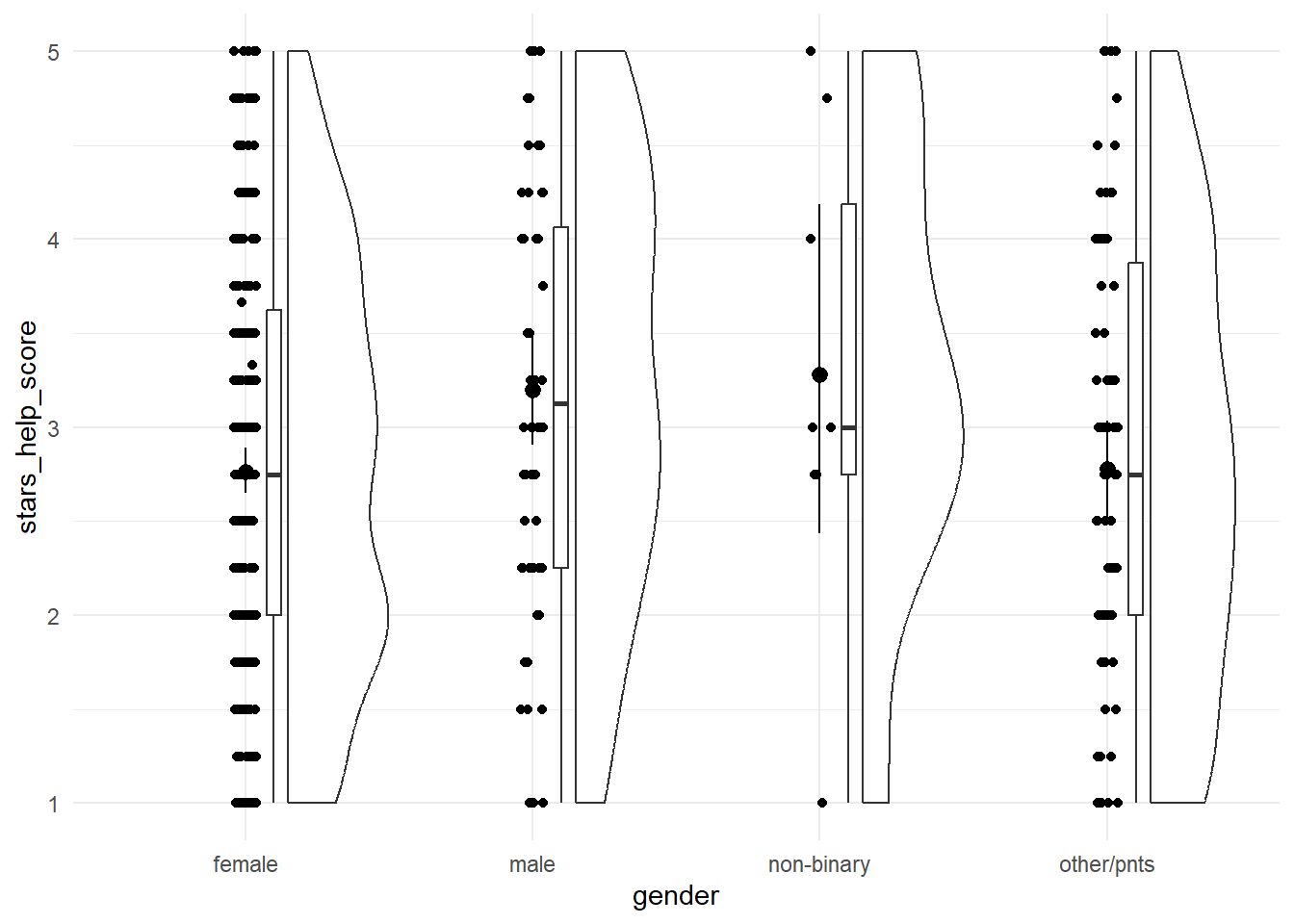

Exercise

Optionally, spruce up this plot with labels and a theme, and some colour contrast for the means and CIs.

Solution

anx_data |> 
  ggplot2::ggplot(aes(x = gender, y = stars_help_score)) + 
  geom_rain() + ## or swap out for geom_violin()!
  stat_summary(fun.data = "mean_cl_boot",
               colour = "darkcyan") +
  ## here's the sprucing
  labs(x = "Gender Identity", y = "STARS Asking for Help Anxiety Score") +
  theme_minimal()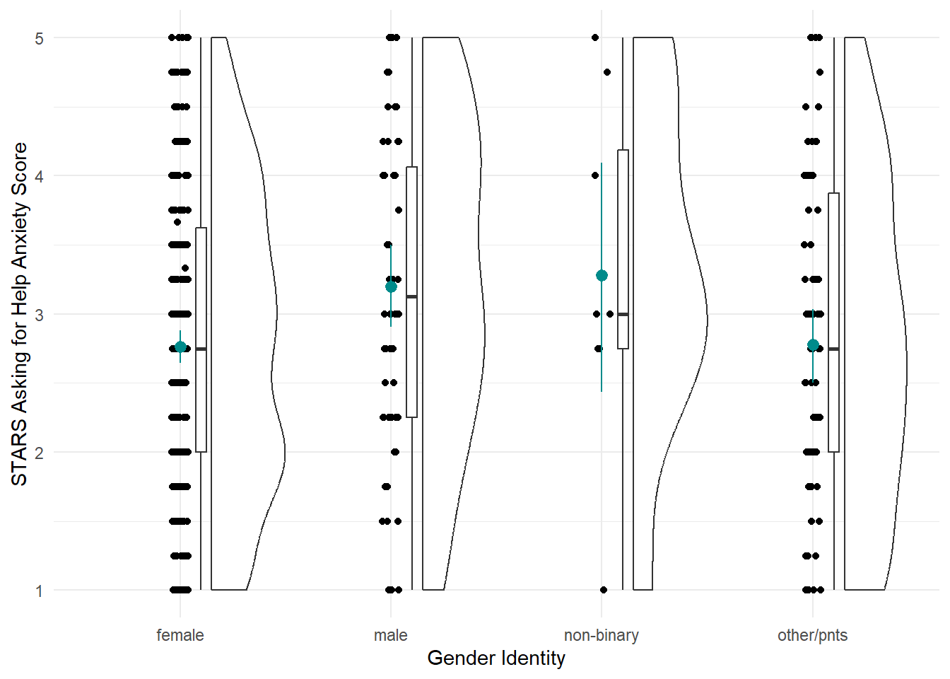

Fit the Model

As mentioned above, this model is taught as a linear model with a categorical predictor. That’s literal: we’re going to use the lm() function to fit the model. It was a bit ago, but we covered the linear model and lm() function in more depth back in Tutorial 06.

Exercise

Follow the steps below to fit and examine the model.

Next up, we need to fit the model. There’s absolutely no difference between this and what we did previously in Tutorial 06, at all, so let’s use the same technique to fit a linear model with STARS Asking for Help subscale score as the outcome and gender as the predictor, and save this model as stars_lm.

stars_lm <- lm(stars_help_score ~ gender, data = anx_data)

Next, again just as we did previously, we can get model fit statistics and an F ratio for the model using broom::glance().

broom::glance(stars_lm)

In discovr_11, though, we see that we can use the anova() function as well. We used this previously to compare models, but given only one model, it will instead compare that model to the null model (i.e. the mean of the outcome). The tutorial also provides code to get an omega effect size.

anova(stars_lm) |> 
  parameters::model_parameters(effectsize_type = "omega")

Finally, we can get a look at the model parameters using broom::tidy(), and see what R has done about our categorical predictor.

broom::tidy(stars_lm, conf.int = TRUE)

To read this output, we need to know a few things about how R deals with categorical predictors by default.

Unless we specify comparisons/contracts, lm() will by default fit a model with the first category as the baseline. What do we mean by the “first”? Here - since the gender variable is a character variable - the first alphabetically. Our categories were female, male, non-binary, and other/pnts, so the first is “female”. (You can see in the plot as well that the categories have been automatically ordered this way.) This means that the intercept represents the mean of the outcome in the baseline group - here, the mean Asking for Help anxiety score in female participants.

The three other three parameter estimates - gendermale, gendernon-binary, and genderother/pnts - each represent the difference in the mean of the outcome between the baseline category and each other category. For example, the b estimate and the rest of the statistics on the gendermale row represent the difference in mean Asking for Help anxiety between female and male participants. The next, gendernon-binary, represents the difference in mean Asking for Help anxiety between female and non-binary participants, and so on.

If this happens to be the comparison you wanted, you’re good to go from here. However, if you wanted different contrasts between groups, then the box below will point you in the right direction.

Contrasts

When they cover ANOVA in second year, UGs are taught to manually write orthogonal contrast weights. We are not going to do that but the whole process is described in the {discovr} tutorial if that’s something you want to do.

Instead, we’re going to use built-in contrasts. The structure generally looks like this:

contrasts(dataset_name$variable_name) <- contr.*(...)

On the left side of this statement, we’re using the contrasts() function to set the contrasts for a particular variable. Notice this is the variable in the dataset, which we’re specifying using $ notation as we’ve seen before. To do this, we assign a pre-set series of contrasts using one of the contr.*() family of functions. Here, the * represents one of a few options, such as contr.sum() (the one we’ll use now), contr.helmert(), etc., and the ... represents some more arguments you may need to add to this function, depending on which one you want. You can get information about all of them by pulling up the help documentation on any of them.

For now, we’re going to use contr.sum(), which requires that we also provide the number of levels (here, four: female, male, non-binary, and other/pnts). There’s a catch, though - we can only set contrasts for factors, so we’ll first need to do something about the gender variable.

Exercise

First, change the character gender variable into a factor. You can do this just for this variable, or optionally use some of the challenge functions from the previous tutorials to change all of the character variables into factors together.

Then, use contr.sum() to set the contrasts for the gender variable.

Solution

Without any fancy extras, we can just change gender into a factor directly - don’t forget to assign the change back to the dataset.

anx_data <- anx_data |> 
  dplyr::mutate(
    gender = factor(gender)
  )

To make sure we don’t have to deal with this again, we can change all of the character variables into factors with the across() + where() tag team from the mutate() tutorial extras.

anx_data <- anx_data |> 
  dplyr::mutate(
    across(where(is.character), factor)
  )

Now that gender is a factor, we can set the contrasts.

contrasts(anx_data$gender) <- contr.sum(4)

Exercise

Fit the model again and get the same parameters table as before.

Solution

Because the underlying gender variable has changed, all we need to do is rerun the exact same code as before, which will now produce output with contrasts.

Just so I can compare them if I want to, I’m going to call this model something different.

stars_contr_lm <- lm(stars_help_score ~ gender, data = anx_data)

papaja::apa_table(papaja::apa_print(stars_contr_lm)$table)

(#tab:unnamed-chunk-21)
Predictor	$b$	95% CI	$t$	$\mathit{df}$	$p$
Intercept	3.01	[2.79, 3.22]	27.05	461	< .001
Gender1	-0.24	[-0.48, -0.01]	-2.01	461	.045
Gender2	0.19	[-0.10, 0.49]	1.29	461	.199
Gender3	0.28	[-0.32, 0.87]	0.92	461	.360

Post-Hoc Tests

If we didn’t have an a priori prediction about the differences between groups, we may decide to instead run post-hoc tests. We can use the function modelbased::estimate_contrasts() to get post-hoc tests by putting in the original model (before we set the contrasts) and telling it which variable to produce the tests for. Confusingly, this argument that does the post-hoc tests is also called contrast = !

Unfortunately, we have a slightly weird problem here. If we just run this command as is, we’ll get something strange in the output:

modelbased::estimate_contrasts(stars_lm, 
                               contrast = "gender")

Notice the unnamed extra column between “Level2” and “Difference”. It appears that the slash in other/pnts has been parsed as a separator, leading to this category being split up into two. TThe results are still readable, but not ideal, so we need to edit our data to remove the forward slash before we carry on with the post-hocs.

In order to resolve this, you know what’s up: string manipulation!! 🎉

Exercise

CHALLENGE: Complete the following steps to update the output.

Change out the “/” in other/pnts for an underscore, so the value reads other_pnts. Do this for all the values in the dataset.
- Hint: You can try stringr::str_replace_all() for a {tidyverse} solution, or if you’re basic like me, have a look at gsub().
Convert the new gender variable back into a factor (as the string manipulation above will have forced it to become character).
Fit the model again and run estimate_contrasts() to get the post-hoc results.

Solution

Parts 1 and 2, done together because they are both within mutate().

{stringr} solution:

anx_data <- anx_data |> 
  dplyr::mutate(
    gender = stringr::str_replace_all(gender, 
                                      pattern = "/", 
                                      replacement = "_") |> 
      factor()
  )

gsub() solution:

anx_data <- anx_data |> 
  dplyr::mutate(
    gender = factor(
      gsub(pattern = "/", 
           replacement = "_", 
           x = gender)
    )
  )

These will do exactly the same thing, so which one you use is completely preference. It’s very useful to know how to do this sort of thing though!

Part 3:

## Refit the model with the newly formatted data
stars_lm <- lm(stars_help_score ~ gender, data = anx_data)

## Finally get the post-hocs!
modelbased::estimate_contrasts(stars_lm, 
                               contrast = "gender")

Factorial Designs

Our next analysis will be factorial design with two categorical predictors, traditionally called a 2x2 independent ANOVA. Although this can certainly be done using lm(), at this point the lm() route becomes a bit burdensome, so we will instead switch to using the {afex} package, which is designed especially for these types of analyses (“afex” stands for “analysis of factorial experiments”). The {discovr} tutorials for this and subsequent similar ANOVA-type analyses demonstrate both {afex} and lm() options, but students are only required to use {afex}.

For our practice today, we’ll look at MCQ question type, and we’ll compare whether mean post-MCQ state anxiety scores are different depending on whether participants have high or low trait anxiety.

Tip

This section is derived from discovr_13, which also has more explanations and advanced techniques.

Fit the Model

First we need to make a change to our dataset - namely, creating the sticsa_trait_cat variable we looked at last week as well.

Exercise

Recode the existing sticsa_trait_score variable into a categorical variable, with “high” values of 2.5 or greater, and “low” values below 2.5. Don’t forget to save this change to your dataset!

Solution

Expensive and sophisticated dplyr::case_when() option:

anx_data <- anx_data |> 
  dplyr::mutate(
    sticsa_trait_cat = dplyr::case_when(
      sticsa_trait_score >= 2.5 ~ "high", 
      sticsa_trait_score < 2.5 ~ "low",
      .default = NA)
  )

Cheap and cheerful ifelse() option:

anx_data <- anx_data |> 
  dplyr::mutate(
    sticsa_trait_cat = ifelse(sticsa_trait_score >= 2.5, "high", "low")
  )

With our categorical predictor in place, we can now fit our model.

Exercise

Follow along with the code below to fit and interpret the model.

The function we’ll use for this and the next analysis as well is afex::aov_4(). The arguments to this function will look extremely familiar - in fact, it looks just about exactly like the way we used the lm() function. The only new thing is the extra element at the end of the function, + (1|id). We can ignore it for now, although we’ll come back to it in the mixed design analysis. The main thing to notice is that if your dataset doesn’t have one, you’ll need a variable that contains ID codes or numbers of some type to use here. This dataset conveniently has anonymous alphanumeric ID codes in a variable called id, but if yours doesn’t, you’d have to add or generate them.

## Store the model
mcq_afx <- afex::aov_4(sticsa_post_state_score ~ mcq*sticsa_trait_cat + (1|id), 
                       data = anx_data)
## Print the model
mcq_afx

Anova Table (Type 3 tests)

Response: sticsa_post_state_score
                Effect     df  MSE          F  ges p.value
1                  mcq 1, 459 0.28       0.68 .001    .412
2     sticsa_trait_cat 1, 459 0.28 202.09 *** .306   <.001
3 mcq:sticsa_trait_cat 1, 459 0.28       0.50 .001    .482
---
Signif. codes:  0 '***' 0.001 '**' 0.01 '*' 0.05 '+' 0.1 ' ' 1

So it seems that there’s a significant main effect of anxiety (no surprise there), but no interaction with MCQ type.

Exercise

CHALLENGE: Imagine you were working with a dataset that didn’t already have ID codes. How could you generate a new id_code variable to use in the {afex} formula, that has a unique value for each row?

Solution

There are so many ways to do this, but here’s two quick ones.

First, you could simply generate a new variable containing the numbers 1 through as many rows as there are in the dataset.

anx_data |> 
  dplyr::mutate(
    id_code = 1:dplyr::n(),
    .before = id
  )

Second, you could use a function to convert the row numbers of the dataset into a variable:

anx_data |> 
  tibble::rowid_to_column(var = "id_code")

Interaction Plot

Besides producing easy-to-read output, one of the handy things about {afex} is that you can quickly generate interaction plots. The afex_plot() function lets you take a model you’ve produced with {afex} and visualise it easily. Since we have one of those to hand (convenient!) let’s have a look.

Minimally, we need to provide the model object, the variable to put on the x-axis, and the “trace”, the variable on separate lines. Unlike with {ggplot}, though, here we need to provide the names of those variables as strings inside quotes.

afex::afex_plot(mcq_afx,
                x = "mcq",
                trace = "sticsa_trait_cat")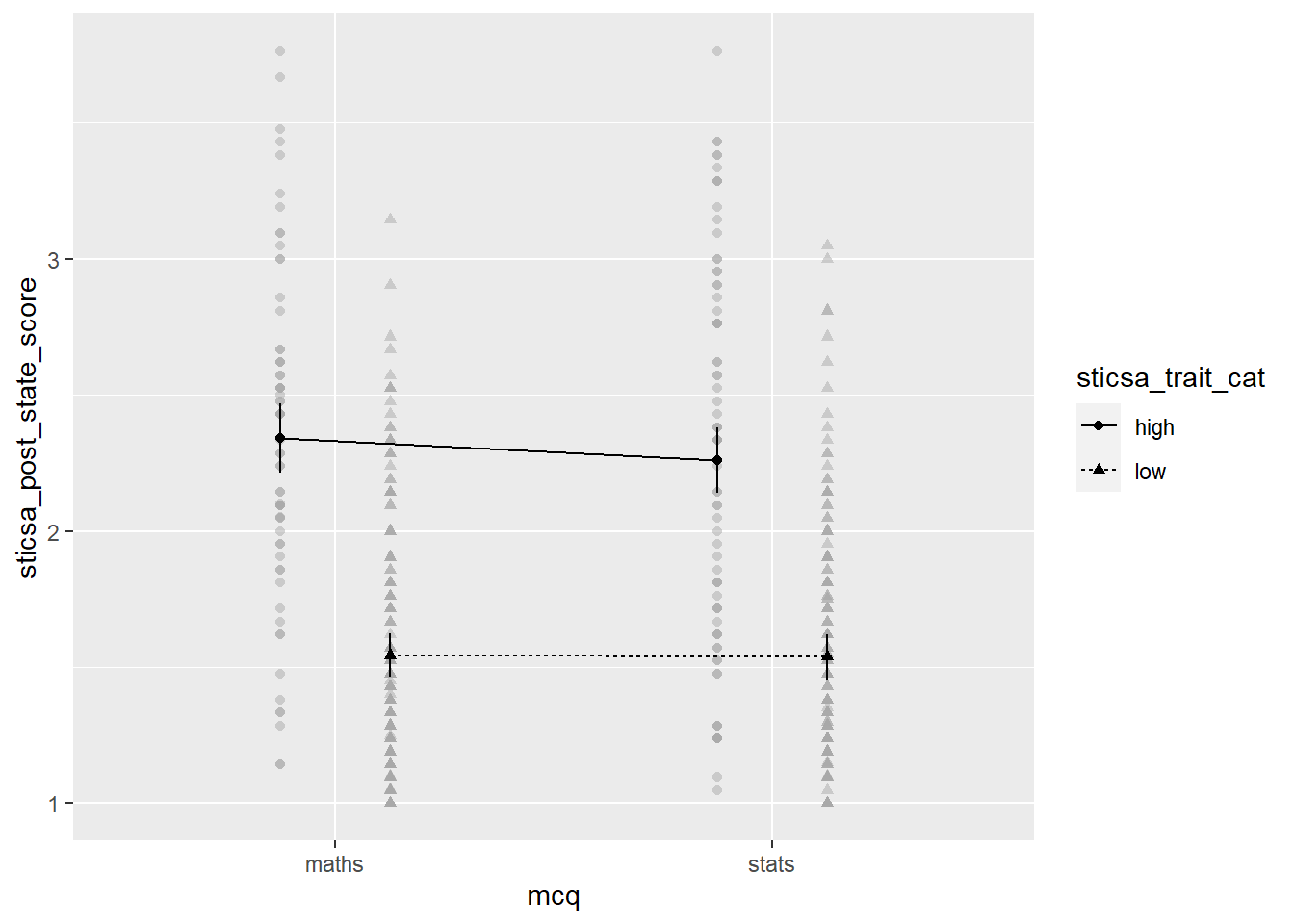

The plot we get for very little work already has a lot of useful stuff. We get means for each combination of groups, with different values on the “trace” variable with different point shapes and connected by different lines. It needs some work, of course, but especially as a quick glimpse at the relationships of interest, it’s a good start!

Exercise

Generate the plot.

CHALLENGE: Use the afex_plot() help documentation and last week’s tutorial on {ggplot2} to clean up this plot and make it presentable.

Solution

Here’s what I went for! There’s a couple small bits left, like the labels on the legend, that I’ll leave to you to work out.

afex::afex_plot(mcq_afx, "mcq", "sticsa_trait_cat",
                legend_title = "STICSA Trait\nAnxiety",
                factor_levels = list(
                  sticsa_cat = c(high = "High",
                                 low = "Low")),
                data_arg = list(
                  position = position_jitterdodge()
                )
                ) +
  scale_x_discrete(name = "Type of MCQ", 
                     labels = c("Maths", "Stats")) +
  scale_y_continuous(name = "STICSA Post-Test State Anxiety",
                     limits = c(1,4),
                     breaks = 1:4) +
  papaja::theme_apa()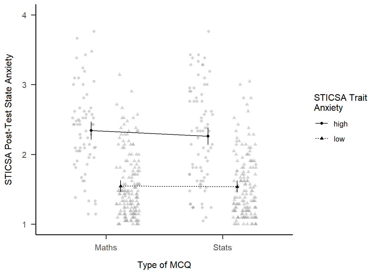

EMMs and Simple Effects

In addition to the plot, we can get get the estimated marginal means (EMMs) for each combination of categories. As with everything, there’s a package for it! Just like with afex_plot(), we provide the model object and the relevant variables to calculate means for.

emmeans::emmeans(mcq_afx, c("mcq", "sticsa_trait_cat"))

 mcq   sticsa_trait_cat emmean     SE  df lower.CL upper.CL
 maths high               2.34 0.0648 459     2.21     2.47
 stats high               2.26 0.0608 459     2.14     2.38
 maths low                1.54 0.0411 459     1.46     1.62
 stats low                1.54 0.0427 459     1.45     1.62

Confidence level used: 0.95

Exercise

Generate the table of estimated marginal means.

CHALLENGE: Turn this estimated marginal means table into a nicely formatted table using kbl() (and, if you feel up for it, pivot_wider()).

Solution

The only information I really want out of this table are the means and confidence intervals. Instead of keeping all the other info, I decided to combine the means and CIs into a single variable using paste0(). The rest is just rearranging, relabelling, and making things look good!

emmeans::emmeans(mcq_afx, c("mcq", "sticsa_trait_cat")) |> 
  ## convert to tibble to work with more easily
  tibble::as_tibble() |> 
  ## concatenate all the info into a new variable and reformat mcq
  dplyr::mutate(
    mean_ci = paste0(round(emmean, 2), " ",
                "[", round(lower.CL, 2), 
                ", ", round(upper.CL, 2), "]"),
    mcq = stringr::str_to_title(mcq)
  ) |> 
  ## keep only categorical vars and new one
  dplyr::select(mcq, sticsa_trait_cat, mean_ci) |> 
  ## reshape
  tidyr::pivot_wider(
    names_from = sticsa_trait_cat,
    values_from = mean_ci
  ) |> 
  ## reorder
  dplyr::select(mcq, low, high) |> 
  kableExtra::kbl(
    col.names = c("MCQ Condition", "Low Anxiety", "High Anxiety"),
    align = "c",
    caption = "STICSA Post-Test State Anxiety means and 95% confidence intervals"
  ) |> 
  kableExtra::kable_classic() |> 
  kableExtra::add_header_above(header = c(" " = 1, 
                               "STICSA Trait Anxiety" = 2))

STICSA Post-Test State Anxiety means and 95% confidence intervals
	STICSA Trait Anxiety
MCQ Condition	Low Anxiety	High Anxiety
Maths	1.54 [1.46, 1.62]	2.34 [2.21, 2.47]
Stats	1.54 [1.45, 1.62]	2.26 [2.14, 2.38]

Finally, we can get tests of the effect between the levels of one variable, within each level of the other. Using the emmeans::joint_tests() function, we can use the model object and the name of the variable we want to split by to get tests within each level of that variable.

emmeans::joint_tests(mcq_afx, "mcq")

Exercise

Produce the same output but the other way round, i.e. for the trait anxiety predictor.

Solution

emmeans::joint_tests(mcq_afx, "sticsa_trait_cat")

Mixed Designs

Tip

This section is derived from discovr_16, which also has more explanations and advanced techniques.

For our final ANOVA-y analysis for today, we’ll look at mixed designs - that is, models with categorical predictors that include at least one independent-measures variable and at least one repeated-measures variable. This is exactly what we’ll do, using STICSA state anxiety timepoint (pre and post) and MCQ type to predict STICSA state anxiety scores. But before we do, we need to look at something we’ve been dancing around in the challenge tasks: at long last, it’s time to tackle pivoting.

Reshaping with `pivot_*()`

For our upcoming analysis, we need to change the way our data are organised in the dataset. We have a repeated measures variable that is currently measured in two variables, namely sticsa_pre_state_score and sticsa_post_state_score. This is how other programmes, like SPSS, also represent repeated measures data, but this is not what we need for R. Instead, we need to reshape our data, so that instead of two separate variables, each with state anxiety scores, we have a single sticsa_state_score variable containing all the scores, with a separate sticsa_time coding variable telling us which timepoint each score comes from, “pre” or “post”. When we’re done, each participant will have two rows in the dataset.

Reshaping in {tidyverse} is typically done with the tidyr::pivot_*() family of functions, which have two star players: pivot_wider() and pivot_longer(). We use generally pivot_wider() when we want to turn rows into columns - which increases the number of columns, and makes the dataset wider - and pivot_longer() when we want to turn columns into rows - which increases the number of rows, and makes the dataset longer. Here, we want to turn columns into rows, and our dataset will actually get longer (we’ll have twice the rows as before!), so it’s pivot_longer() we need.

Partying with pivot

Need help with pivoting? Me too, like all the time. Run vignette("pivot") in the Console for an absolutely indispensable guide through both types of pivoting with a wealth of easily adaptable examples and code.

For this analysis, we’re going to start by select()ing only the variables we actually need for the analysis, just to keep things as simple as possible. Next up is pivot_longer() to reshape the dataset. Minimally we have to specify the columns to pivot (using <tidyselect>, of course!), and where the names and values go to.

In this case, the columns we want to pivot are the ones containing “state” - that is, sticsa_pre_state_score and sticsa_post_state_score. The names of these variables are moved to a new variable, sticsa_time, using the names_to = argument - this variable now contains those names as values about timepoint (pre or post). The values that those variables previously contained, which for both variables were STICSA state anxiety scores, are moved to a new variable, sticsa_state_score, using the values_to = argument. Looking at the id and other variables, we can see that, as expected, there are now two rows for each participant, one “pre” and one “post”. Result!

anx_data |> 
  dplyr::select(id, contains(c("sticsa", "mcq"))) |> 
  tidyr::pivot_longer(cols = contains("state"),
                      names_to = "sticsa_time",
                      values_to = "sticsa_state_score")

As will not surprise anyone in the slightest, I (JM) suggest one final step, if you’re willing to once again wander dangerously close to regular expressions. The final names_pattern argument allows me to specify a portion of the variable names to be moved in names_to, instead of the entire variable name. We can see that the names sticsa_pre_state_score and sticsa_post_state_score contain only one important element: either “pre” or “post”, between the first and second underscores. The brackets in the regular expression below capture this portion of each name and keep only that string in the new sticsa_time variable, which makes the new variable much easier to work with and read.

anx_data |> 
  dplyr::select(id, contains(c("sticsa", "mcq"))) |> 
  tidyr::pivot_longer(cols = contains("state"),
                      names_to = "sticsa_time",
                      values_to = "sticsa_state_score",
                      names_pattern = ".*?_(.*?)_.*")

Exercise

Reshape the dataset as above and assign to a new dataset name, anx_data_long, lest we overwrite all our data with this much smaller and reshaped dataset!

Hint: It’s fine to copy the code above, especially if you’re short on time, but you’ll learn and understand the code much better if you type it out instead of copying it.

Solution

anx_data_long <- anx_data |> 
  dplyr::select(id, contains(c("sticsa", "mcq"))) |> 
  tidyr::pivot_longer(cols = contains("state"),
                      names_to = "sticsa_time",
                      values_to = "sticsa_state_score",
                      names_pattern = ".*?_(.*?)_.*")

Exercise

CHALLENGE: How can you read the regular expression .*?_(.*?)_.*? If you’re not sure, try putting into regex101.com for some help (without the quotes).

Solution

Disclaimer: This is an extremely nontechnical explanation, and is meant to capture the gist of what the regex does (as I understand it!) rather than to be technically accurate.

This expression really only contains four elements: .*?, .*, (), and _. The last one, the underscore, is just a literal underscore, so all we need to worry about are the other three.

. is a very handy token in regex that means “any character” (except line terminators). Literally anything: letters, numbers, punctuation, symbols, whitespace, etc. * is a quantifier, expressing how many of the preceding element to match, and means “match between zero and unlimited times”. So, we can read .* as “any character any number of times, including none.” * is a “greedy” quantifier, which means it will match as many times as possible.

So, what about .*?? The only new element is the ?, which combines with * to create a “lazy” quantifier, matching as few times as possible. So, we can read .*? as “any character any number of times, including none, but as few as possible.”

Finally, the brackets () are a capturing group - a portion of the expression we want to single out. In this case, it denotes the portion of the string that we want to actually use as the data in our new sticsa_time variable.

So how can we read .*?_(.*?)_.*? Let’s compare to an example string, sticsa_pre_state_score.

.*?_ matches any number of characters as few times as possible until it encounters an underscore. This captures the sticsa_ portion of the example string.
(.*?)_ matches any number of characters as few times as possible until it encounters the next underscore. This matches the pre_ portion of the example string, with the brackets singling out the capturing group of interest, namely the string “pre”.
.* matches any number of characters for the rest of the string. This matches the state_score portion of the example string.

So, why didn’t I type "sticsa_(.*)_state_score"? It would have worked just as well (try it!). In a word, generalisability. .*?_(.*?)_.* will get the element between the first and second underscores in any string, whereas "sticsa_(.*)_state_score" will only work for these particular variables. That’s a matter of personal choice and style, but I almost always prefer the generalisable way if possible, because I know it’ll be easier to adapt the next time round.

If you like this kind of thing, bookmark regex101 and consider reading vignette("regular-expressions")!

Fit the Model

Exercise

Follow along with the code below to fit and interpret the model.

To fit our model, we’ll use a very similar formula that was just saw for factorial designs. We’re using the new sticsa_state_score as the outcome, with mcq (the independent-measures variable) and sticsa_time (the repeated-measures variable), and their interaction, as predictors. The key difference is in the last element of our formula, which is now + (sticsa_time|id). In other words, I’ve replaced the 1 in + (1|id) with the repeated element(s) of the model.

# fit the model:
anx_mcq_afx <- anx_data_long |> 
  afex::aov_4(sticsa_state_score ~ mcq*sticsa_time + (sticsa_time|id),
              data = _)

anx_mcq_afx

Anova Table (Type 3 tests)

Response: sticsa_state_score
           Effect     df  MSE      F   ges p.value
1             mcq 1, 461 0.68   0.60  .001    .438
2     sticsa_time 1, 461 0.08   0.01 <.001    .907
3 mcq:sticsa_time 1, 461 0.08 4.28 *  .001    .039
---
Signif. codes:  0 '***' 0.001 '**' 0.01 '*' 0.05 '+' 0.1 ' ' 1

Main Effects

We can see from the output above that neither main effects are significant. However, that might not always be the case, so there’s a couple ways we can investigate the effect.

The first is to get estimated marginal means (EMMs) for all levels of the main effect, which we can do using the emmeans::emmeans() function. It might be useful to save the output in a new object so you can refer to (or report!) it easily.

Second, we can visualise the effect easily using afex::afex_plot() and only specifying one variable on the x-axis. I haven’t worried about any additional zhooshing, except to whack on a theme.

mcq_emm <- emmeans::emmeans(anx_mcq_afx, ~mcq, model = "multivariate")
mcq_emm

 mcq   emmean     SE  df lower.CL upper.CL
 maths   1.75 0.0383 461     1.68     1.83
 stats   1.79 0.0386 461     1.72     1.87

Results are averaged over the levels of: sticsa_time 
Confidence level used: 0.95

afex::afex_plot(anx_mcq_afx,
                x = "mcq") +
  papaja::theme_apa()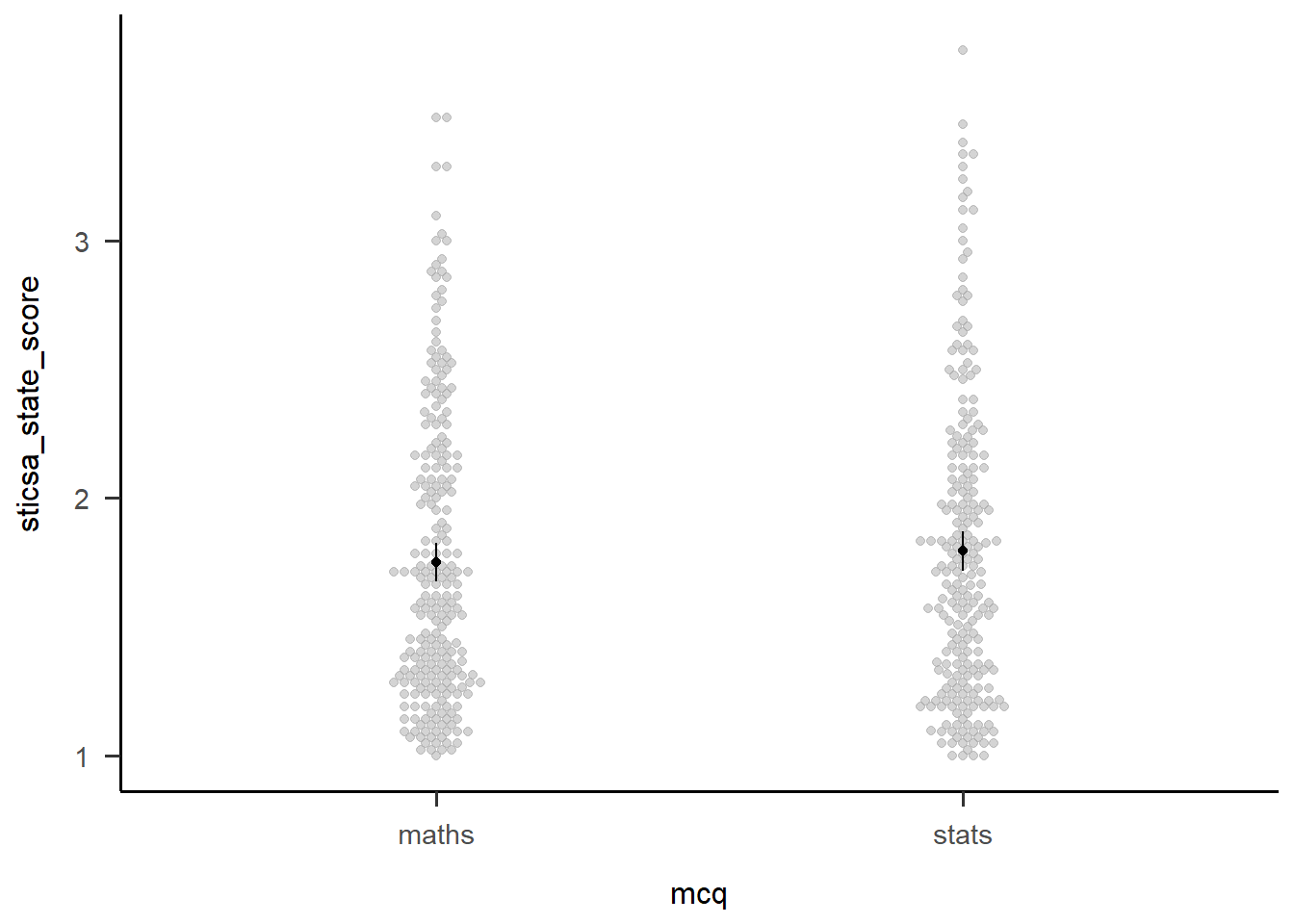

Exercise

Following the example above, get EMMs and a plot for the main effect of sticsa_time.

Solution

You can almost exactly adapt the code above, but watch out for the warning on the plot:

Warning: Panel(s) show within-subjects factors, but not within-subjects error bars.
For within-subjects error bars use: error = "within"

This seems very sensible!

time_emm <- emmeans::emmeans(anx_mcq_afx, ~sticsa_time, model = "multivariate")
time_emm

 sticsa_time emmean     SE  df lower.CL upper.CL
 pre           1.77 0.0281 461     1.72     1.83
 post          1.77 0.0295 461     1.72     1.83

Results are averaged over the levels of: mcq 
Confidence level used: 0.95

afex::afex_plot(anx_mcq_afx,
                x = "sticsa_time",
                error = "within") +
  papaja::theme_apa()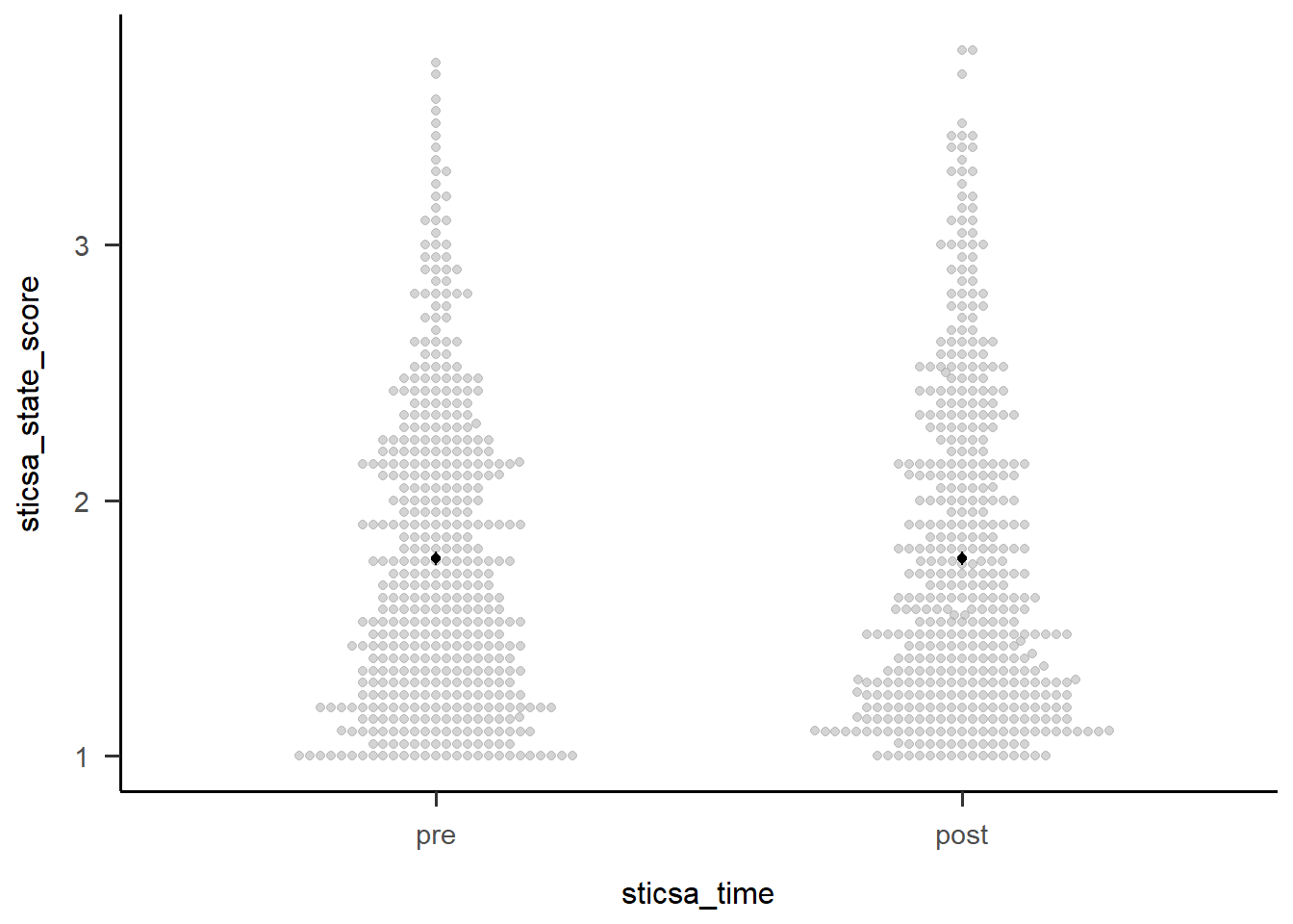

Two-Way Interactions

The first thing we might want to do with an interaction is break it apart to understand what’s happening. We can start out with this by getting a table of EMMs just like we did above. These are slightly more interesting than those above, but only just (I can’t make much of these without a plot!).

We could also use emmeans::estimate_contrast() to break down the interaction…except that there’s only the one 2x2 interaction here, so all this gives us is an identical result to the interaction effect in the overall model. For other designs with more levels, the output compares 2x2 combinations of conditions to better understand what’s happening.

anx_mcq_emm <- emmeans::emmeans(anx_mcq_afx, ~c(mcq, sticsa_time), model = "multivariate")
anx_mcq_emm

 mcq   sticsa_time emmean     SE  df lower.CL upper.CL
 maths pre           1.73 0.0395 461     1.65     1.81
 stats pre           1.81 0.0398 461     1.73     1.89
 maths post          1.77 0.0416 461     1.69     1.85
 stats post          1.78 0.0419 461     1.69     1.86

Confidence level used: 0.95

emmeans::contrast(
  anx_mcq_emm,
  interaction = c(mcq = "trt.vs.ctrl", sticsa_time = "trt.vs.ctrl"),
  ref = 2,
  adjust = "holm"
  )

 mcq_trt.vs.ctrl sticsa_time_trt.vs.ctrl estimate     SE  df t.ratio p.value
 maths - stats   pre - post               -0.0784 0.0379 461  -2.070  0.0390

But of course, the main thing we want to see is the interaction plot! Just as we did before, we can use afex_plot() to quickly get the bones of the plot and finally see what the hell is going on.

afex::afex_plot(anx_mcq_afx,
                x = "sticsa_time",
                trace = "mcq",
                error = "none") +
  papaja::theme_apa()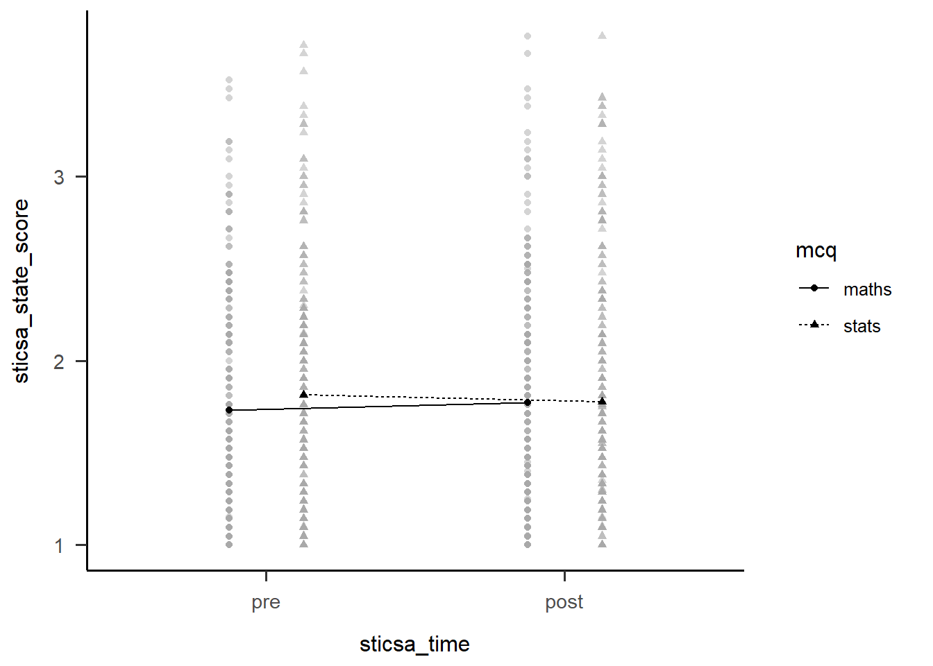

Before we go too far into zhooshing this plot, which we’ve already had a go at, let’s have a look at {papaja}’s entry into the automatically-making-cool-plots race. To get started, we’ll set up a plot giving the data, ID variable, dependent variable (outcome), and factors (predictors):

papaja::apa_beeplot(
  data = anx_data_long,
  id = "id",
  dv = "sticsa_state_score",
  factors = c("sticsa_time", "mcq")
)

Not bad for a first effort! I like that this version shows how the points are dispersed. I don’t like a good few other things: the weird axes, the strange amount of whitespace, the lack of connecting lines to help judge the interaction.

Which one to use? Honestly, it depends on personal preference, the data, the journal requirements, and how comfortable you feel with each function.

Exercise

Generate the plot with papaja::apa_beeplot().

CHALLENGE: Zhoosh up this plot to get it at least within spitting distance of nicely formatted.

Hint: Use the {papaja} help documentation!

Solution

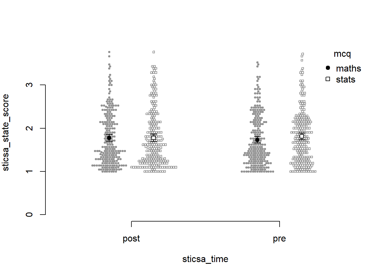
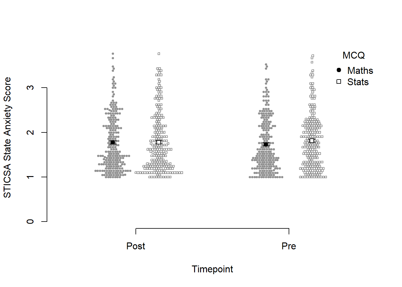
papaja::apa_beeplot(
  data = anx_data_long,
  id = "id",
  dv = "sticsa_state_score",
  factors = c("sticsa_time", "mcq"),
  dispersion = within_subjects_conf_int,
  ylab = "STICSA State Anxiety Score",
  xlab = "Timepoint",
  args_x_axis = list(
    labels = c("Post", "Pre")
  ),
  args_legend = list(
    title = "MCQ",
    legend = c("Maths", "Stats")
  )
)

Reproducibility Report: Part Two

We conducted a variety of tests and have many, many results, woohoo! Time to make sure all this code is reproducible!

The second part of the report covers the reproducibility of the numerical results, inferential conclusions, figures, and tables produced by the analysis. We have discussed all the issues covered in these sections in previous tutorials, so it is time to put everything we have learned together.

Numerical results - Tutorial 6
Inferential conclusions - Tutorial 6
Figures - Tutorial 8
Tables - Tutorial 6, Tutorial 7

Exercises

For the remainder of the session you can choose the activity you find most appealing.

Option 1: Continue working

Start a new script, loading the data and packages as we did in the beginning. Then, choose one the analyses we conducted above, or conduct a different analysis of your choice. Generate a table with descriptive statistics, summarising your variables the variables on interest, write a paragraph summarising the results of your chose analysis, and generate a figure to go with the results. As you are working, go through the reproducibility report template and note any points you are having trouble with.

Option 2: Work on one of your own projects

Using what we have learned today and in the course as a whole, glam up the analysis of a project your are currently working on. Go through the reproducibility report template and try to pinpoint the areas where you can improve your code.

Option 3: Conduct a reproducibility check on a published study

If you’d like to try doing a reproducibility check, Reny will send you a link to a randomly chosen paper via email.

You can continue working on these exercises on your own time. When you are finished, if you’d like some feedback, share your code and other materials with Reny.

Submitting Your Work

You have completed your manuscript draft, your code is beautifully formatted and commented, and you’ve put together an exquisite readme file and you want to share your materials with Reny. What should you do?

You should definitely upload:

Your data
Your code
Readme file and data dictionaries

These are pretty much essential. If the data and code are not freely available, the analysis cannot be reproduced.

In addition, it would be nice to:

Upload the rendered document (if using Quarto)
Upload the manuscript itself on a pre-print server

These are not essential, but would make me very, very happy.

For more information on how to share your materials, have a look at the Sussex Data Repository. OSF is a very popular repository, but we should make use of our own in-house resources when we can.

Final Thoughts

This is the end of the R training course - well done! Making it all the way here is quite an accomplishment.

The best thing you can do from here is to start using R as much as possible. You don’t have to swear off all other programmes (although you could 👀), but choose a task that you need to do anyway and trying doing it in R instead. Like any language, it will get smoother and easier with regular use.

By the way, don’t feel discouraged if you encounter lots of errors, or have to go back and look up code from your notes, these tutorials, the Internet, etc. That’s not only completely normal, it’s a really useful part of the process. Don’t expect to just sit down and bash out hundreds of lines of code from memory. Neither of us (Jennifer and Reny) do that! Coding anything, new tasks or familiar, always takes time, reference to resources, patience, and a lot of error resolution.

Finally, we are always available to answer any R-related questions you have. Both Jennifer and Reny love talking about and helping others with R, so if you have something in mind you’d like to do or learn, give either of us a shout.

Congratulations once again, and good luck from here on your jouRney!

Footnotes

I think this issue has now been fixed, but still it’s wild it was ever a thing.↩︎
JM: Speak for yourself! I love that kind of thing 😂↩︎

Overview

Reproducibility Certification

Setup

Packages

Data

Codebook

Reproducibility Report: Part One

Section 1: Reproducibility of Data Processing

Question 1

Question 5

Section 2: Reproducibility of Analysis Environment

Questions 5 & 6

Section 3: Reproducibility of Analysis Pipeline

Question 3

Question 4

Question 5

ANOVA Speedrun

One-Way ANOVA

Plot

Fit the Model

Factorial Designs

Fit the Model

Interaction Plot

EMMs and Simple Effects

Mixed Designs

Reshaping with pivot_*()

Fit the Model

Main Effects

Two-Way Interactions

Reproducibility Report: Part Two

Exercises

Option 1: Continue working

Option 2: Work on one of your own projects

Option 3: Conduct a reproducibility check on a published study

Submitting Your Work

Final Thoughts

Footnotes

Reshaping with `pivot_*()`