08: Analysis

Overview

This tutorial is a speedrun of how to run and report a variety of analyses that are commonly used for undergraduate dissertation projects at the University of Sussex, based on a survey of supervisors in summer 2023.

Important

This is not a statistics tutorial, so interpretation of the following models will be only cursory. For a complete explanation of the statistical concepts and interpretation, refer to the {discovr} tutorials that correspond to the following sections:

Categorical Predictors
- Comparing Several Means (One-Way ANOVA): discovr_11
- Factorical Designs: discovr_13
- Mixed Designs: discovr_16
Moderation: discovr_10
Mediation: discovr_10

Using the {discovr} tutorials

Prof Andy Field’s {discovr} tutorials provide detailed walkthroughs of both the R code and the statistical concepts of a variety of statistical analyses. They are a good place to look first to understand what your UG supervisees or advisees have been taught on a particular topic.

To install the tutorials, run the following in the Console. Note that this is not necessary for the live workshop Cloud workspaces, which already have the tutorials installed.

if(!require(remotes)){
  install.packages('remotes')
}

remotes::install_github("profandyfield/discovr")

The {discovr} tutorials are built in {learnr}, an interactive platform for learning and running R code. So, unlike the tutorial you’re currently reading, they must be run inside an R session.

To start a tutorial, open any project and click on the Tutorial tab in the Environment pane. Scroll down to the tutorial you want and click the “Start Tutorial ▶️” button to load the tutorial.

Because {discovr} tutorials run within R, you don’t need to use any external documents; you can write and run R code within the tutorial itself. However, I strongly recommend that whenever you work with these tutorials, you write and run your code in a separate document, otherwise you will have no record of the code and output.

Setup

Packages

There are a lot of packages that we will make our way through today. The key ones are, naturally, {tidyverse}; {afex} for factorial designs; {ggrain} for raincloud plots; {lavaan} for mediation; and {papaja} for pretty formatting and reporting.

Exercise

Load the packages.

Solution

library(tidyverse)
library(afex)
library(ggrain)
library(lavaan)
library(papaja)

Data

Today we’re continuing to work with the dataset courtesy of fantastic Sussex colleague Jenny Terry. This dataset contains real data about statistics and maths anxiety. For these latter two tutorials, I’ve created averaged scores for each overall scale and subscale, and dropped the individual items.

Exercise

Read in the dataset and save it in a new object, anx_data.

On the Cloud, you can read in this dataset from the data folder using here::here().

Elsewhere, you can download the dataset, or copy the dataset URL, from the Data and Workbooks page.

Solution

Read in from file:

anx_data <- readr::read_csv(here::here("data/anx_scores_data.csv"))

Read in from URL:

anx_data <- readr::read_csv("https://raw.githubusercontent.com/drmankin/practicum/master/data/anx_data.csv")

Codebook

There’s quite a bit in this dataset, so you will need to refer to the codebook below for a description of all the variables.

Dataset Info Recap

This study explored the difference between maths and statistics anxiety, widely assumed to be different constructs. Participants completed the Statistics Anxiety Rating Scale (STARS) and Maths Anxiety Rating Scale - Revised (R-MARS), as well as modified versions, the STARS-M and R-MARS-S. In the modified versions of the scales, references to statistics and maths were swapped; for example, the STARS item “Studying for an examination in a statistics course” became the STARS-M item “Studying for an examination in a maths course”; and the R-MARS item “Walking into a maths class” because the R-MARS-S item “Walking into a statistics class”.

Participants also completed the State-Trait Inventory for Cognitive and Somatic Anxiety (STICSA). They completed the state anxiety items twice: once before, and once after, answering a set of five MCQ questions. These MCQ questions were either about maths, or about statistics; each participant only saw one of the two MCQ conditions.

Important

For learning purposes, I’ve randomly generated some additional variables to add to the dataset containing info on distribution channel, consent, gender, and age. Especially for the consent variable, don’t worry: all the participants in this dataset did consent to the original study. I’ve simulated and added this variable in later to practice removing participants.

Variable	Type	Description	Values
id	Categorical	Unique ID code	NA
distribution	Categorical	Channel through which the study was completed, either as a preview (before real data collection) or anonymous genuine responses. Note that this variable has been randomly generated and does NOT reflect genuine responses.	"preview" or "anonymous"
consent	Categorical	Whether the participant read and consented to participate. Note that this variable has been randomly generated and does NOT reflect genuine responses; all participants in this dataset did originally consent to participate.	"Yes" or "No"
gender	Categorical	Gender identity. Note that this variable has been randomly generated and does NOT reflect genuine responses.	"female", "male", "non-binary", or "other/pnts". "pnts" is an abbreviation for "Prefer not to say".
age	Numeric	Age in years. Note that this variable has been randomly generated and does NOT reflect genuine responses.	18 - 99
mcq	Categorical	Independent variable for MCQ question condition, whether the participant saw MCQ questions about mathematics or statistics.	"maths" or "stats"
stars_test_score	Numeric	Averaged score on the Test Anxiety subscale of the Statistics Anxiety Rating Scale (STARS)	1 (low anxiety) to 5 (high anxiety)
stars_int_score	Numeric	Averaged score on the Interpretation Anxiety subscale of the Statistics Anxiety Rating Scale (STARS)	1 (low anxiety) to 5 (high anxiety)
stars_help_score	Numeric	Averaged score on the Asking for Help subscale of the Statistics Anxiety Rating Scale (STARS)	1 (low anxiety) to 5 (high anxiety)
stars_m_test_score	Numeric	Averaged score on the Test Anxiety subscale of the Statistics Anxiety Rating Scale - Maths (STARS-M), a modified version of the STARS with all references to maths replaced with statistics.	1 (low anxiety) to 5 (high anxiety)
stars_m_int_score	Numeric	Averaged score on the Interpretation Anxiety subscale of the Statistics Anxiety Rating Scale - Maths (STARS-M), a modified version of the STARS with all references to maths replaced with statistics.	1 (low anxiety) to 5 (high anxiety)
stars_m_help_score	Numeric	Averaged score on the Asking for Help subscale of the Statistics Anxiety Rating Scale - Maths (STARS-M), a modified version of the STARS with all references to maths replaced with statistics.	1 (low anxiety) to 5 (high anxiety)
rmars_test_score	Numeric	Averaged score on the Test Anxiety subscale of the Revised Maths Anxiety Rating Scale (R-MARS)	1 (low anxiety) to 5 (high anxiety)
rmars_num_score	Numeric	Averaged score on the Numerical Task Anxiety subscale of the Revised Maths Anxiety Rating Scale (R-MARS)	1 (low anxiety) to 5 (high anxiety)
rmars_course_score	Numeric	Averaged score on the Course Anxiety subscale of the Revised Maths Anxiety Rating Scale (R-MARS)	1 (low anxiety) to 5 (high anxiety)
rmars_s_test_score	Numeric	Averaged score on the Test Anxiety subscale of the Revised Maths Anxiety Rating Scale - Statistics (R-MARS-S), a modified version of the MARS with all references to maths replaced with statistics.	1 (low anxiety) to 5 (high anxiety)
rmars_s_num_score	Numeric	Averaged score on the Numerical Anxiety subscale of the Revised Maths Anxiety Rating Scale - Statistics (R-MARS-S), a modified version of the MARS with all references to maths replaced with statistics.	1 (low anxiety) to 5 (high anxiety)
rmars_s_course_score	Numeric	Averaged score on the Course Anxiety subscale of the Revised Maths Anxiety Rating Scale - Statistics (R-MARS-S), a modified version of the MARS with all references to maths replaced with statistics.	1 (low anxiety) to 5 (high anxiety)
sticsa_trait_score	Numeric	Averaged score on the Trait Anxiety subscale of the State-Trait Inventory for Cognitive and Somatic Anxiety.	1 (not at all) to 4 (very much so)
sticsa_pre_state_score	Numeric	Averaged score on the State Anxiety subscale of the State-Trait Inventory for Cognitive and Somatic Anxiety, pre-MCQ.	1 (not at all) to 4 (very much so)
sticsa_post_state_score	Numeric	Averaged score on the State Anxiety subscale of the State-Trait Inventory for Cognitive and Somatic Anxiety, post-MCQ.	1 (not at all) to 4 (very much so)
mcq_score	Numeric	Total (summed) score on the MCQ questions.	0 (all incorrect) to 5 (all correct)

If you have some experience with R, you are welcome to instead use another dataset that you are familiar with or are keen to explore. However, remember that anything you upload to Posit Cloud is visible to all workspace admins, so keep GDPR in mind.

Categorical Predictors

We’ll begin by looking at several examples of models with categorical predictors. Traditionally, these are all different types of “ANOVA” (ANalysis Of VAriance), but research methods teaching at Sussex teaches all of these models in the framework of the general linear model.

Comparing Several Means

Our first model will be linear model with a categorical predictor with more than two categories - traditionally a “one-way independent ANOVA”. For our practice today, we’ll look at the differences in the STARS Asking for Help subscore by gender.

Tip

This section is derived from discovr_11, which also has more explanations and advanced techniques.

Plot

Let’s start by visualising our variables. The discovr tutorial also includes code for a table of means and CIs, which we won’t cover here.

Exercise

Use what we covered in the last tutorial to create a violin or raincloud plot (your choice) with means and CIs. Optionally, spruce up your plot with labels and a theme.

Solution

anx_data |> 
  ggplot2::ggplot(aes(x = gender, y = stars_help_score)) + 
  geom_rain() + ## or swap out for geom_violin()!
  stat_summary(fun.data = "mean_cl_boot") +
  ## here's the sprucing
  labs(x = "Gender Identity", y = "STARS Asking for Help Anxiety Score") +
  theme_minimal()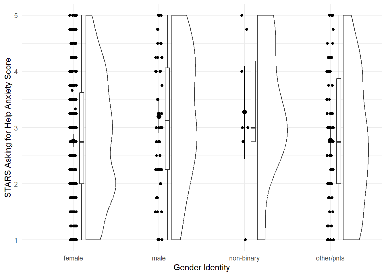

Fit the Model

As mentioned above, this model is taught as a linear model with a categorical predictor. That’s literal: we’re going to use the lm() function to fit the model. It was a bit ago, but we covered the linear model and lm() function in more depth back in Tutorial 04.

Unfortunately, we’ll need to make a quick change to our data beforehand.

Exercise

Change out the “/” in the value other/pnts for an underscore, so the value reads other_pnts.

Hint: You can try stringr::str_replace_all() for a {tidyverse} solution, or if you’re basic like me, have a look at gsub().

Solution

{stringr} solution:

anx_data <- anx_data |> 
  dplyr::mutate(
    gender = stringr::str_replace_all(gender, 
                                      pattern = "/", 
                                      replacement = "_")
  )

gsub() solution:

anx_data <- anx_data |> 
  dplyr::mutate(
    gender = gsub("/", "_", gender)
  )

These will do exactly the same thing, so which one you use is completely preference. It’s very useful to know how to do this sort of thing though!

Exercise

Follow the steps below to fit and examine the model.

Next up, we need to fit the model. There’s absolutely no difference between this and what we did previously in Tutorial 04, at all, so let’s use the same technique to fit a linear model with STARS Asking for Help subscale score as the outcome and gender as the predictor, and save this model as stars_lm.

stars_lm <- lm(stars_help_score ~ gender, data = anx_data)

Next, again just as we did previously, we can get model fit statistics and an F ratio for the model using broom::glance().

broom::glance(stars_lm)

In discovr_11, though, we see that we can use the anova() function as well. We used this previously to compare models, but given only one model, it will instead compare that model to the null model (i.e. the mean of the outcome). The tutorial also provides code to get an omega effect size.

anova(stars_lm) |> 
  parameters::model_parameters(effectsize_type = "omega")

Finally, we can get a look at the model parameters using broom::tidy(), and see what R has done about our categorical predictor.

broom::tidy(stars_lm, conf.int = TRUE)

To read this output, we need to know a few things about how R deals with categorical predictors by default.

Unless we specify comparisons/contracts, lm() will by default fit a model with the first category as the baseline. What do we mean by the “first”? Here, the first alphabetically. Our categories were female, male, non-binary, and other_pnts, so the first is “female”. (You can see in the plot as well that the categories have been automatically ordered this way.) This means that the intercept represents the mean of the outcome in the baseline group - here, the mean Asking for Help anxiety score in female participants.

The three other three parameter estimates - gendermale, gendernon-binary, and genderother_pnts - each represent the difference in the mean of the outcome between the baseline category and each other category. For example, the b estimate and the rest of the statistics on the gendermale row represent the difference in mean Asking for Help anxiety between female and male participants. The next, gendernon-binary, represents the difference in mean Asking for Help anxiety between female and non-binary participants, and so on.

Contrasts

When they cover this week in second year, UGs are taught to manually write orthogonal contrast weights. We are not going to do that but the whole process is described in the {discovr} tutorial if that’s something you want to do.

Instead, we’re going to use built-in contrasts. The structure generally looks like this:

contrasts(dataset_name$variable_name) <- contr.*(...)

On the left side of this statement, we’re using the contrasts() function to set the contrasts for a particular variable. Notice this is the variable in the dataset, which we’re specifying using $ notation as we’ve seen before. To do this, we assign a pre-set series of contrasts using one of the contr.*() family of functions. Here, the * represents one of a few options, such as contr.sum() (the one we’ll use now), contr.helmert(), etc., and the ... represents some more arguments you may need to add to this function, depending on which one you want. You can get information about all of them by pulling up the help documentation on any of them.

For now, we’re going to use contr.sum(), which requires that we also provide the number of levels (here, four: female, male, non-binary, and other_pnts). There’s a catch, though - we can only set contrasts for factors, so we’ll first need to do something about the gender variable.

Exercise

First, change the character gender variable into a factor. You can do this just for this variable, or optionally use some of the challenge functions from the last tutorials to change all of the character variables into factors together.

Then, use contr.sum() to set the contrasts for the gender variable.

Solution

Without any fancy extras, we can just change gender into a factor directly - don’t forget to assign the change back to the dataset.

anx_data <- anx_data |> 
  dplyr::mutate(
    gender = factor(gender)
  )

To make sure we don’t have to deal with this again, we can change all of the character variables into factors with the across() + where() tag team from the last tutorial.

anx_data <- anx_data |> 
  dplyr::mutate(
    across(where(is.character), factor)
  )

Now that gender is a factor, we can set the contrasts.

contrasts(anx_data$gender) <- contr.sum(4)

Exercise

Fit the model again and get the same parameters table as before.

Solution

Because the underlying gender variable has changed, all we need to do is rerun the exact same code as before, which will now produce output with contrasts.

Just so I can compare them if I want to, I’m going to call this model something different.

stars_contr_lm <- lm(stars_help_score ~ gender, data = anx_data)

papaja::apa_table(papaja::apa_print(stars_contr_lm)$table)

(#tab:unnamed-chunk-16)
Predictor	$b$	95% CI	$t$	$\mathit{df}$	$p$
Intercept	3.01	[2.79, 3.22]	27.05	461	< .001
Gender1	-0.24	[-0.48, -0.01]	-2.01	461	.045
Gender2	0.19	[-0.10, 0.49]	1.29	461	.199
Gender3	0.28	[-0.32, 0.87]	0.92	461	.360

Post-Hoc Tests

If we didn’t have an a priori prediction about the differences between groups, we may decide to instead run post-hoc tests. We can use the function modelbased::estimate_contrasts() to get post-hoc tests by putting in the original model (before we set the contrasts) and telling it which variable to produce the tests for. Confusingly, this argument is also called contrast = !

modelbased::estimate_contrasts(stars_lm, 
                               contrast = "gender")

What about ANCOVA?

The procedures for including a covariate in the linear model aren’t too complex, but the additional work to be done - testing independence of the covariate, changing the type of F-statistic, checking homogeneity of regression slopes, and so on - are just a bit much for this tutorial. If you are Keen to include a covariate, check out the very thorough discovr_12 for a detailed walkthrough.

Factorial Designs

Our next analysis will be factorial design with two categorical predictors, traditionally called a 2x2 independent ANOVA. Although this can certainly be done using lm(), at this point the lm() route becomes a bit burdensome, so we will instead switch to using the {afex} package, which is designed especially for these types of analyses (“afex” stands for “analysis of factorial experiments”). The {discovr} tutorials for this and subsequent similar ANOVA-type analyses demonstrate both {afex} and lm() options, but students are only required to use {afex}.

For our practice today, we’ll look at again at gender, but this time with male and female participants only, and we’ll compare whether their post-MCQ state anxiety scores are different depending on whether have high or low trait anxiety.

Tip

This section is derived from discovr_13, which also has more explanations and advanced techniques.

Fit the Model

First we need to make a change to our dataset - namely, creating the sticsa_trait_cat variable we looked at last week as well.

Exercise

Recode the existing sticsa_trait_score variable into a categorical variable, with “high” values of 2.5 or greater, and “low” values below 2.5. Don’t forget to save this change to your dataset!

Solution

Expensive and sophisticated dplyr::case_when() option:

anx_data <- anx_data |> 
  dplyr::mutate(
    sticsa_trait_cat = dplyr::case_when(
      sticsa_trait_score >= 2.5 ~ "high", 
      sticsa_trait_score < 2.5 ~ "low",
      .default = NA)
  )

Cheap and cheerful ifelse() option:

anx_data <- anx_data |> 
  dplyr::mutate(
    sticsa_trait_cat = ifelse(sticsa_trait_score >= 2.5, "high", "low")
  )

With our categorical predictor in place, we can now fit our model.

Exercise

Follow along with the code below to fit and interpret the model.

The function we’ll use for this and the next analysis as well is afex::aov_4(). The arguments to this function will look extremely familiar - in fact, it looks just about exactly like the way we used the lm() function. The only new thing is the extra element at the end of the function, + (1|id). We can ignore it for now, although we’ll come back to it in the mixed design analysis. The main thing to notice is that if your dataset doesn’t have one, you’ll need a variable that contains ID codes or numbers of some type to use here. This dataset conveniently has anonymous alphanumeric ID codes in a variable called id, but if yours doesn’t, you’d have to add or generate them.

## Store the model
mcq_afx <- afex::aov_4(sticsa_post_state_score ~ mcq*sticsa_trait_cat + (1|id), 
                       data = anx_data)
## Print the model
mcq_afx

Anova Table (Type 3 tests)

Response: sticsa_post_state_score
                Effect     df  MSE          F  ges p.value
1                  mcq 1, 459 0.28       0.68 .001    .412
2     sticsa_trait_cat 1, 459 0.28 202.09 *** .306   <.001
3 mcq:sticsa_trait_cat 1, 459 0.28       0.50 .001    .482
---
Signif. codes:  0 '***' 0.001 '**' 0.01 '*' 0.05 '+' 0.1 ' ' 1

So it seems that there’s a significant main effect of anxiety (no surprise there), but no interaction with MCQ type.

Exercise

CHALLENGE: Imagine you were working with a dataset that didn’t already have ID codes. How could you generate a new id_code variable to use in the {afex} formula, that has a unique value for each row?

Solution

There are so many ways to do this, but here’s two quick ones.

First, you could simply generate a new variable containing the numbers 1 through as many rows as there are in the dataset.

anx_data |> 
  dplyr::mutate(
    id_code = 1:dplyr::n(),
    .before = id
  )

Second, you could use a function to convert the row numbers of the dataset into a variable:

anx_data |> 
  tibble::rowid_to_column(var = "id_code")

Interaction Plot

Besides producing easy-to-read output, one of the handy things about {afex} is that you can quickly generate interaction plots. The afex_plot() function lets you take a model you’ve produced with {afex} and visualise it easily. Since we have one of those to hand (convenient!) let’s have a look.

Minimally, we need to provide the model object, the variable to put on the x-axis, and the “trace”, the variable on separate lines. Unlike with {ggplot}, though, here we need to provide the names of those variables as strings inside quotes.

afex::afex_plot(mcq_afx,
                x = "mcq",
                trace = "sticsa_trait_cat")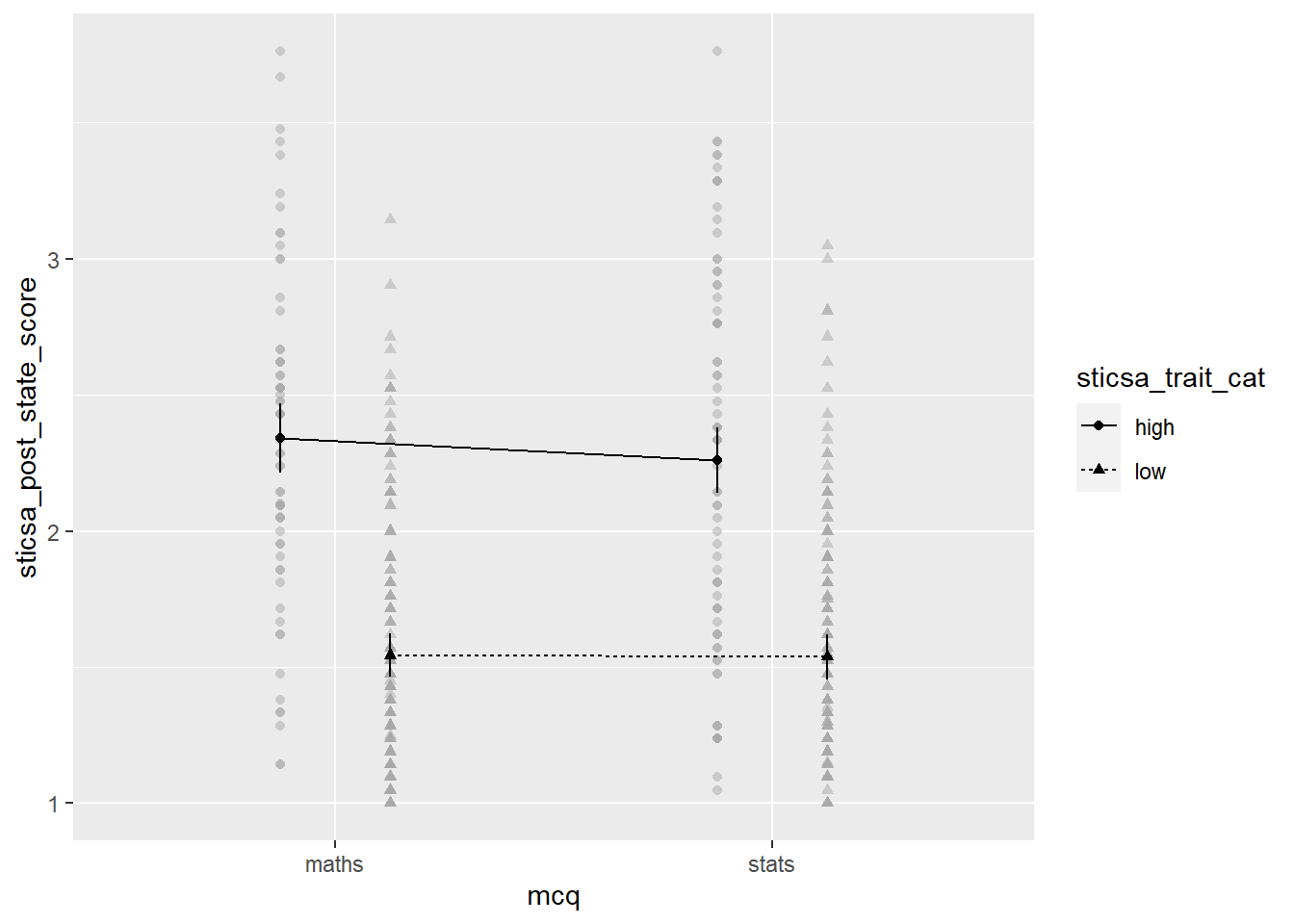

The plot we get for very little work already has a lot of useful stuff. We get means for each combination of groups, with different values on the “trace” variable with different point shapes and connected by different lines. It needs some work, of course, but especially as a quick glimpse at the relationships of interest, it’s a good start!

Exercise

Generate the plot.

CHALLENGE: Use the afex_plot() help documentation and last week’s tutorial on {ggplot2} to clean up this plot and make it presentable.

Solution

Here’s what I went for! There’s a couple small bits left, like the labels on the legend, that I’ll leave to you to work out.

afex::afex_plot(mcq_afx, "mcq", "sticsa_trait_cat",
                legend_title = "STICSA Trait\nAnxiety",
                factor_levels = list(
                  sticsa_cat = c(high = "High",
                                 low = "Low")),
                data_arg = list(
                  position = position_jitterdodge()
                )
                ) +
  scale_x_discrete(name = "Type of MCQ", 
                     labels = c("Maths", "Stats")) +
  scale_y_continuous(name = "STICSA Post-Test State Anxiety",
                     limits = c(1,4),
                     breaks = 1:4) +
  papaja::theme_apa()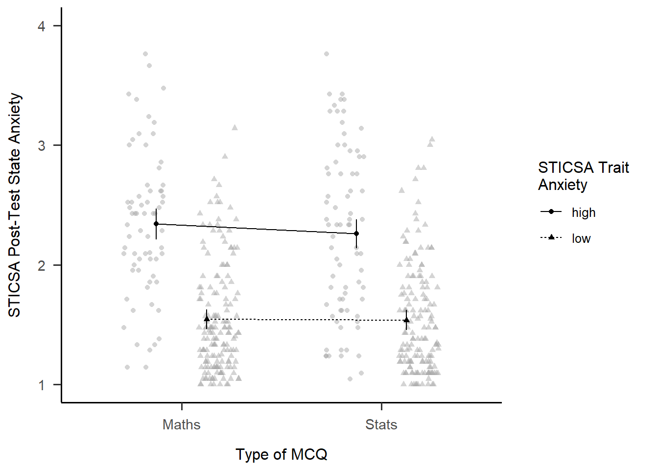

EMMs

In addition to the plot, we can get get the actual means for each combination of categories. As with everything, there’s a package for it! Just like with afex_plot(), we provide the model object and the relevant variables to calculate means for.

emmeans::emmeans(mcq_afx, c("mcq", "sticsa_trait_cat"))

 mcq   sticsa_trait_cat emmean     SE  df lower.CL upper.CL
 maths high               2.34 0.0648 459     2.21     2.47
 stats high               2.26 0.0608 459     2.14     2.38
 maths low                1.54 0.0411 459     1.46     1.62
 stats low                1.54 0.0427 459     1.45     1.62

Confidence level used: 0.95

Exercise

Generate the table of estimated marginal means.

CHALLENGE: Turn this estimated marginal means table into a nicely formatted table using kbl() (and, if you feel up for it, pivot_wider()).

Solution

The only information I really want out of this table are the means and confidence intervals. Instead of keeping all the other info, I decided to combine the means and CIs into a single variable using paste0(). The rest is just rearranging, relabelling, and making things look good!

emmeans::emmeans(mcq_afx, c("mcq", "sticsa_trait_cat")) |> 
  ## convert to tibble to work with more easily
  tibble::as_tibble() |> 
  ## concatenate all the info into a new variable and reformat mcq
  dplyr::mutate(
    mean_ci = paste0(round(emmean, 2), " ",
                "[", round(lower.CL, 2), 
                ", ", round(upper.CL, 2), "]"),
    mcq = stringr::str_to_title(mcq)
  ) |> 
  ## keep only categorical vars and new one
  dplyr::select(mcq, sticsa_trait_cat, mean_ci) |> 
  ## reshape
  tidyr::pivot_wider(
    names_from = sticsa_trait_cat,
    values_from = mean_ci
  ) |> 
  ## reorder
  dplyr::select(mcq, low, high) |> 
  kableExtra::kbl(
    col.names = c("MCQ Condition", "Low Anxiety", "High Anxiety"),
    align = "c",
    caption = "STICSA Post-Test State Anxiety means and 95% confidence intervals"
  ) |> 
  kableExtra::kable_classic() |> 
  kableExtra::add_header_above(header = c(" " = 1, 
                               "STICSA Trait Anxiety" = 2))

STICSA Post-Test State Anxiety means and 95% confidence intervals
	STICSA Trait Anxiety
MCQ Condition	Low Anxiety	High Anxiety
Maths	1.54 [1.46, 1.62]	2.34 [2.21, 2.47]
Stats	1.54 [1.45, 1.62]	2.26 [2.14, 2.38]

Simple Effects

Finally, we can get tests of the effect between the levels of one variable, within each level of the other. Using the emmeans::joint_tests() function, we can use the model object and the name of the variable we want to split by to get tests within each level of that variable.

emmeans::joint_tests(mcq_afx, "mcq")

Exercise

Produce the same output but the other way round, i.e. for the trait anxiety predictor.

Solution

emmeans::joint_tests(mcq_afx, "sticsa_trait_cat")

Mixed Designs

Tip

This section is derived from discovr_16, which also has more explanations and advanced techniques.

For our final ANOVA-y analysis for today, we’ll look at mixed designs - that is, models with categorical predictors that include at least one independent-measures variable and at least one repeated-measures variable. This is exactly what we’ll do, using STICSA state anxiety timepoint (pre and post) and MCQ type to predict STICSA state anxiety scores. But before we do, we need to look at something we’ve been dancing around in the challenge tasks: at long last, it’s time to tackle pivoting.

Reshaping with `pivot_*()`

For our upcoming analysis, we need to change the way our data are organised in the dataset. We have a repeated measures variable that is currently measured in two variables, namely sticsa_pre_state_score and sticsa_post_state_score. This is how other programmes, like SPSS, also represent repeated measures data, but this is not what we need for R. Instead, we need to reshape our data, so that instead of two separate variables, each with state anxiety scores, we have a single sticsa_state_score variable containing all the scores, with a separate sticsa_time coding variable telling us which timepoint each score comes from, “pre” or “post”. When we’re done, each participant will have two rows in the dataset.

Reshaping in {tidyverse} is typically done with the tidyr::pivot_*() family of functions, which have two star players: pivot_wider() and pivot_longer(). We use generally pivot_wider() when we want to turn rows into columns, and pivot_longer() when we want to turn columns into rows. Here, we want to turn columns into rows, and our dataset will actually get longer (we’ll have twice the rows as before!), so it’s pivot_longer() we need.

Partying with pivot

Need help with pivoting? Me too, like all the time. Run vignette("pivot") in the Console for an absolute indispensable guide through both types of pivoting with a wealth of easily adaptable examples and code.

For this analysis, I’m going to start by select()ing only the variables I actually need for the analysis, just to keep things as simple as possible. Next up is pivot_longer() to reshape the dataset. Minimally we have to specify the columns to pivot (using <tidyselect>, of course!), and where the names and values go to.

In this case, the columns I want to pivot are the ones containing “state” - that is, sticsa_pre_state_score and sticsa_post_state_score. The names of these variables are moved to a new variable, sticsa_time, using the names_to = argument - this variable now contains those names as values about timepoint (pre or post). The values that those variables previously contained, which for both variables were STICSA state anxiety scores, are moved to a new variable, sticsa_state_score, using the values_to = argument. Looking at the id and other variables, we can see that, as expected, there are now two rows for each participant, one “pre” and one “post”. Result!

anx_data |> 
  dplyr::select(id, contains(c("sticsa", "mcq"))) |> 
  tidyr::pivot_longer(cols = contains("state"),
                      names_to = "sticsa_time",
                      values_to = "sticsa_state_score")

I’d suggest one final step, if you’re willing to wander dangerously close to regular expressions. The final names_pattern argument allows me to specify a portion of the variable names to be moved in names_to, instead of the entire variable name. We can see that the names sticsa_pre_state_score and sticsa_post_state_score contain only one important element: either “pre” or “post”, between the first and second underscores. The brackets in the regular expression capture this portion of each name and keep only that string in the new sticsa_time variable, which makes the new variable much easier to work with and read.

anx_data |> 
  dplyr::select(id, contains(c("sticsa", "mcq"))) |> 
  tidyr::pivot_longer(cols = contains("state"),
                      names_to = "sticsa_time",
                      values_to = "sticsa_state_score",
                      names_pattern = ".*?_(.*?)_.*")

Exercise

Reshape the dataset as above and assign to a new dataset name, anx_data_long, lest we overwrite all our data with this much smaller and reshaped dataset!

Hint: It’s fine to copy the code above, especially if you’re short on time, but you’ll learn and understand the code much better if you type it out instead of copying it.

Solution

anx_data_long <- anx_data |> 
  dplyr::select(id, contains(c("sticsa", "mcq"))) |> 
  tidyr::pivot_longer(cols = contains("state"),
                      names_to = "sticsa_time",
                      values_to = "sticsa_state_score",
                      names_pattern = ".*?_(.*?)_.*")

Exercise

CHALLENGE: How can you read the regular expression .*?_(.*?)_.*? If you’re not sure, try putting into regex101.com for some help (without the quotes).

Solution

Disclaimer: This is an extremely nontechnical explanation, and is meant to capture the gist of what the regex does (as I understand it!) rather than to be technically accurate.

This expression really only contains four elements: .*?, .*, (), and _. The last one, the underscore, is just a literal underscore, so all we need to worry about are the other three.

. is a very handy token in regex that means “any character” (except line terminators). Literally anything: letters, numbers, punctuation, symbols, whitespace, etc. * is a quantifier, expressing how many of the preceding element to match, and means “match between zero and unlimited times”. So, we can read .* as “any character any number of times, including none.” * is a “greedy” quantifier, which means it will match as many times as possible.

So, what about .*?? The only new element is the ?, which combines with * to create a “lazy” quantifier, matching as few times as possible. So, we can read .*? as “any character any number of times, including none, but as few as possible.”

Finally, the brackets () are a capturing group - a portion of the expression we want to single out. In this case, it denotes the portion of the string that we want to actually use as the data in our new sticsa_time variable.

So how can we read .*?_(.*?)_.*? Let’s compare to an example string, sticsa_pre_state_score.

.*?_ matches any number of characters as few times as possible until it encounters an underscore. This captures the sticsa_ portion of the example string.
(.*?)_ matches any number of characters as few times as possible until it encounters the next underscore. This matches the pre_ portion of the example string, with the brackets singling out the capturing group of interest, namely the string “pre”.
.* matches any number of characters for the rest of the string. This matches the state_score portion of the example string.

So, why didn’t I type "sticsa_(.*)_state_score"? It would have worked just as well (try it!). In a word, generalisability. .*?_(.*?)_.* will get the element between the first and second underscores in any string, whereas "sticsa_(.*)_state_score" will only work for these particular variables. That’s a matter of personal choice and style, but I almost always prefer the generalisable way if possible, because I know it’ll be easier to adapt the next time round.

If you like this kind of thing, bookmark regex101 and consider reading vignette("regular-expressions")!

Fit the Model

Exercise

Follow along with the code below to fit and interpret the model.

To fit our model, we’ll use a very similar formula that was just saw for factorial designs. We’re using the new sticsa_state_score as the outcome, with mcq (the independent-measures variable) and sticsa_time (the repeated-measures variable), and their interaction, as predictors. The key difference is in the last element of our formula, which is now + (sticsa_time|id). In other words, I’ve replaced the 1 in + (1|id) with the repeated element(s) of the model.

# fit the model:
anx_mcq_afx <- anx_data_long |> 
  afex::aov_4(sticsa_state_score ~ mcq*sticsa_time + (sticsa_time|id),
              data = _)

anx_mcq_afx

Anova Table (Type 3 tests)

Response: sticsa_state_score
           Effect     df  MSE      F   ges p.value
1             mcq 1, 461 0.68   0.60  .001    .438
2     sticsa_time 1, 461 0.08   0.01 <.001    .907
3 mcq:sticsa_time 1, 461 0.08 4.28 *  .001    .039
---
Signif. codes:  0 '***' 0.001 '**' 0.01 '*' 0.05 '+' 0.1 ' ' 1

Main Effects

We can see from the output above that neither main effects are significant. However, that might not always be the case, so there’s a couple ways we can investigate the effect.

The first is to get estimated marginal means (EMMs) for all levels of the main effect, which we can do using the emmeans::emmeans() function. It might be useful to save the output in a new object so you can refer to (or report!) it easily.

Second, we can visualise the effect easily using afex::afex_plot() and only specifying one variable on the x-axis. I haven’t worried about any additional zhooshing, except to whack on a theme.

mcq_emm <- emmeans::emmeans(anx_mcq_afx, ~mcq, model = "multivariate")
mcq_emm

 mcq   emmean     SE  df lower.CL upper.CL
 maths   1.75 0.0383 461     1.68     1.83
 stats   1.79 0.0386 461     1.72     1.87

Results are averaged over the levels of: sticsa_time 
Confidence level used: 0.95

afex::afex_plot(anx_mcq_afx,
                x = "mcq") +
  papaja::theme_apa()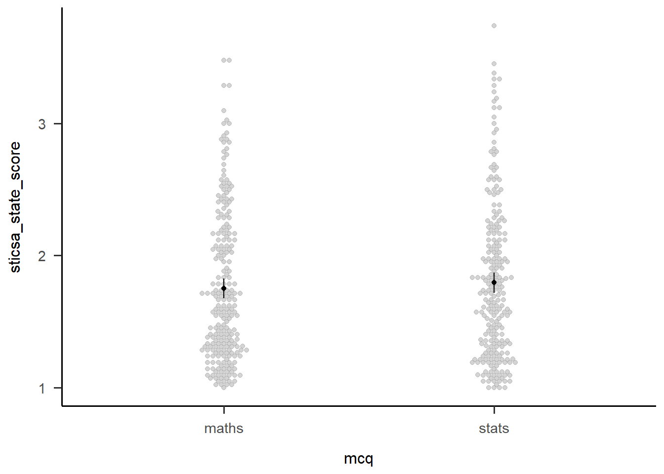

Exercise

Following the example above, get EMMs and a plot for the main effect of sticsa_time.

Solution

You can almost exactly adapt the code above, but watch out for the warning on the plot:

Warning: Panel(s) show within-subjects factors, but not within-subjects error bars.
For within-subjects error bars use: error = "within"

This seems very sensible!

time_emm <- emmeans::emmeans(anx_mcq_afx, ~sticsa_time, model = "multivariate")
time_emm

 sticsa_time emmean     SE  df lower.CL upper.CL
 pre           1.77 0.0281 461     1.72     1.83
 post          1.77 0.0295 461     1.72     1.83

Results are averaged over the levels of: mcq 
Confidence level used: 0.95

afex::afex_plot(anx_mcq_afx,
                x = "sticsa_time",
                error = "within") +
  papaja::theme_apa()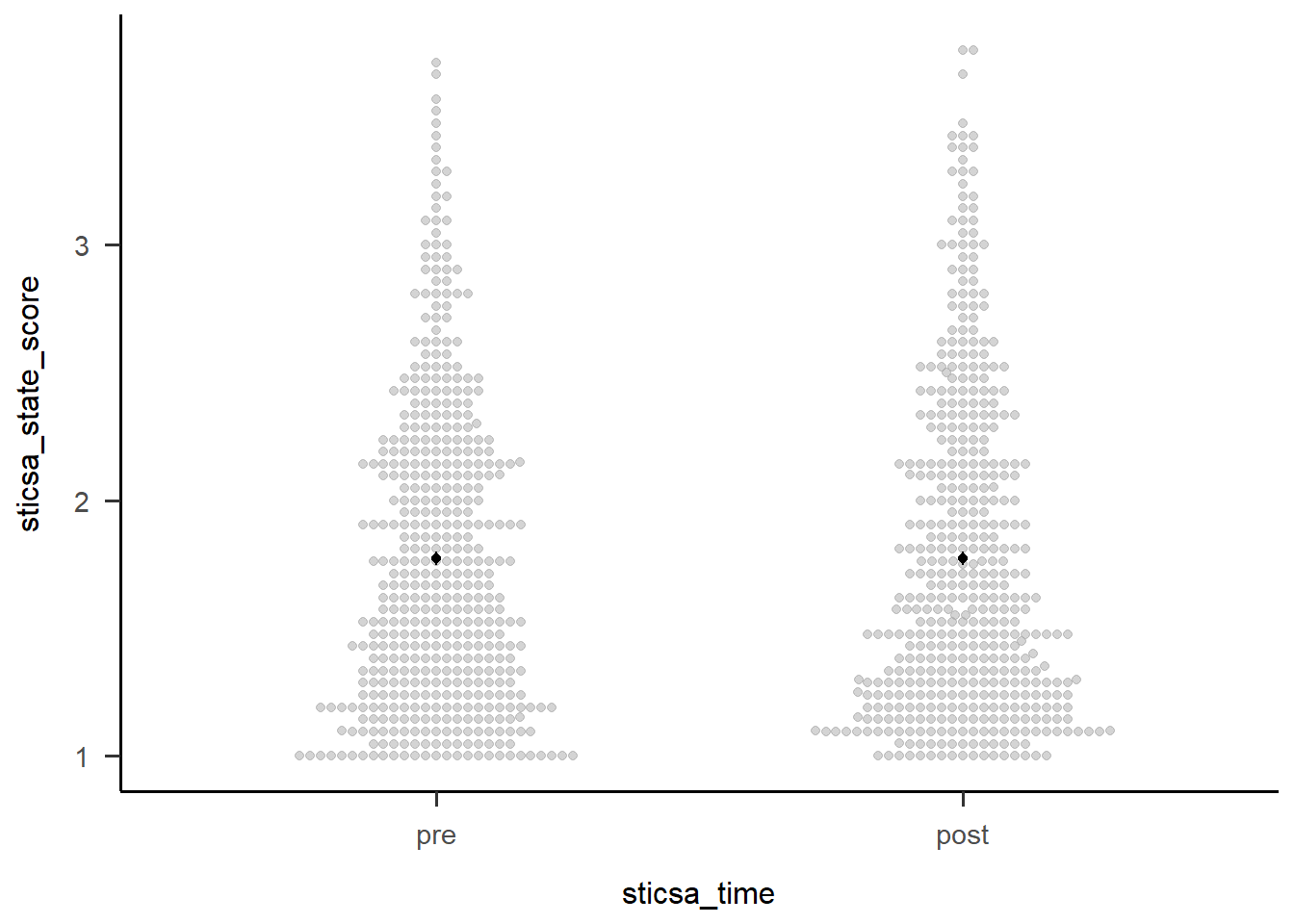

Two-Way Interactions

The first thing we might want to do with an interaction is break it apart to understand what’s happening. We can start out with this by getting a table of EMMs just like we did above. These are slightly more interesting than those above, but only just (I can’t make much of these without a plot!).

We could also use emmeans::estimate_contrast() to break down the interaction…except that there’s only the one 2x2 interaction here, so all this gives us is an identical result to the interaction effect in the overall model. For other designs with more levels, the output compares 2x2 combinations of conditions to better understand what’s happening.

anx_mcq_emm <- emmeans::emmeans(anx_mcq_afx, ~c(mcq, sticsa_time), model = "multivariate")
anx_mcq_emm

 mcq   sticsa_time emmean     SE  df lower.CL upper.CL
 maths pre           1.73 0.0395 461     1.65     1.81
 stats pre           1.81 0.0398 461     1.73     1.89
 maths post          1.77 0.0416 461     1.69     1.85
 stats post          1.78 0.0419 461     1.69     1.86

Confidence level used: 0.95

emmeans::contrast(
  anx_mcq_emm,
  interaction = c(mcq = "trt.vs.ctrl", sticsa_time = "trt.vs.ctrl"),
  ref = 2,
  adjust = "holm"
  )

 mcq_trt.vs.ctrl sticsa_time_trt.vs.ctrl estimate     SE  df t.ratio p.value
 maths - stats   pre - post               -0.0784 0.0379 461  -2.070  0.0390

But of course, the main thing we want to see is the interaction plot! Just as we did before, we can use afex_plot() to quickly get the bones of the plot and finally see what the hell is going on.

afex::afex_plot(anx_mcq_afx,
                x = "sticsa_time",
                trace = "mcq",
                error = "none") +
  papaja::theme_apa()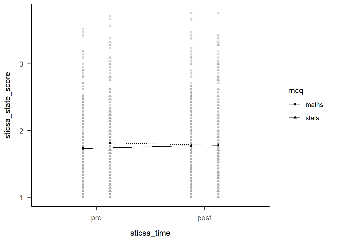

Before we go too far into zhooshing this plot, which we’ve already had a go at, let’s have a look at {papaja}’s entry into the automatically-making-cool-plots race. To get started, we’ll set up a plot giving the data, ID variable, dependent variable (outcome), and factors (predictors):

papaja::apa_beeplot(
  data = anx_data_long,
  id = "id",
  dv = "sticsa_state_score",
  factors = c("sticsa_time", "mcq")
)

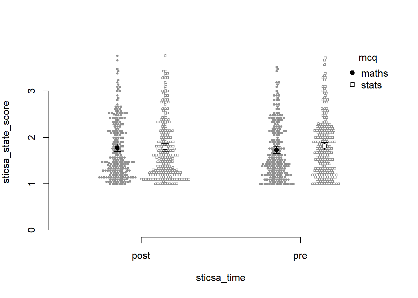
Not bad for a first effort! I like that this version shows how the points are dispersed. I don’t like a good few other things: the weird axes, the strange amount of whitespace, the lack of connecting lines to help judge the interaction.

Which one to use? Honestly, it depends on personal preference, the data, the journal requirements, and how comfortable you feel with each function.

Exercise

Generate the plot with papaja::apa_beeplot().

CHALLENGE: Zhoosh up this plot to get it at least within spitting distance of nicely formatted.

Hint: Use the {papaja} help documentation!

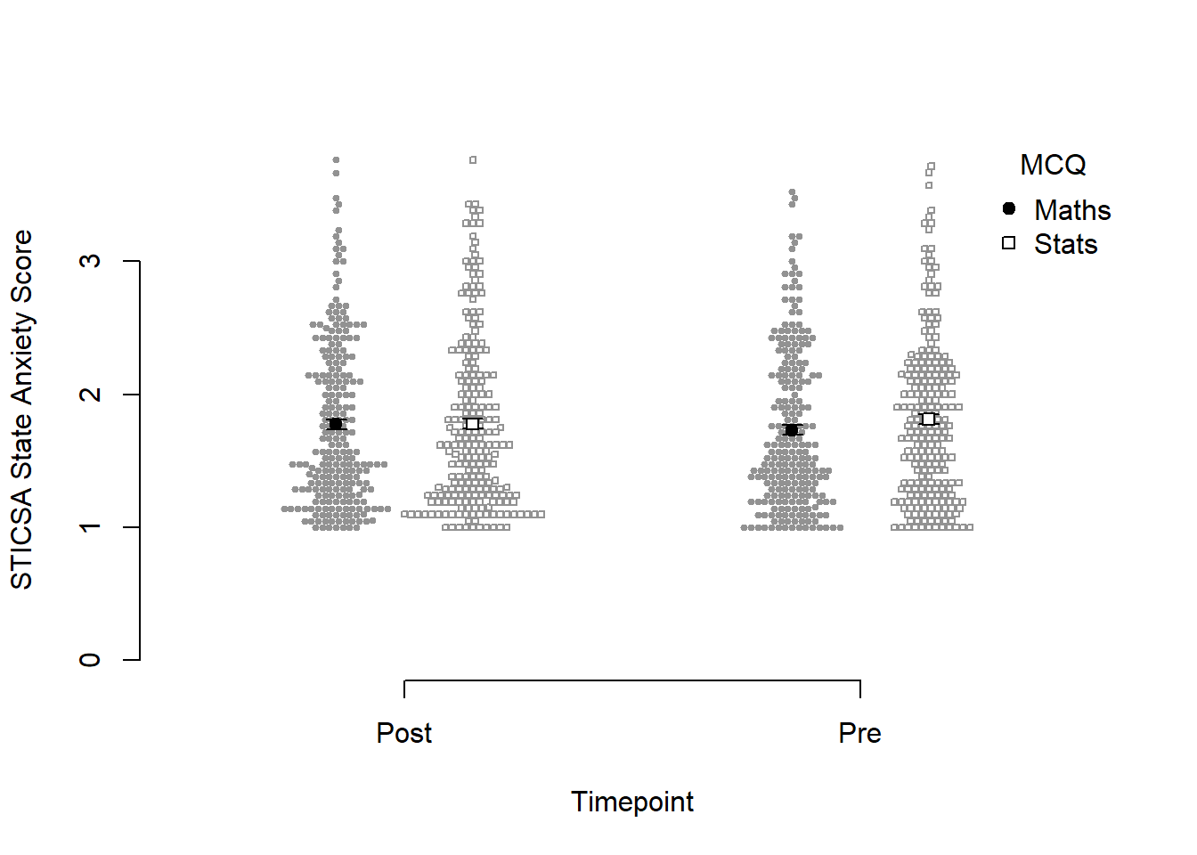
Solution

papaja::apa_beeplot(
  data = anx_data_long,
  id = "id",
  dv = "sticsa_state_score",
  factors = c("sticsa_time", "mcq"),
  dispersion = within_subjects_conf_int,
  ylab = "STICSA State Anxiety Score",
  xlab = "Timepoint",
  args_x_axis = list(
    labels = c("Post", "Pre")
  ),
  args_legend = list(
    title = "MCQ",
    legend = c("Maths", "Stats")
  )
)

Continuous Predictors

Right, had enough of factors? Me too. We’re moving on to models with categorical predictors, which we cover in two broad areas: mediation and moderation.

Mediation

Tip

This section is derived from discovr_10, which also has more explanations and advanced techniques.

Mediation models follow a classic structure. A predictor, X, has some relationship with the outcome, Y; this is the direct effect, c. The mediation route is the hypothesised mechanism by way of which X has its relationship in Y, either in whole or in part. The a and b paths in the model below represent the mediation route via the mediator, M.

flowchart LR
      X -- Path a --> M[M: Mediator] -- Path b--> Y
      X[X: Predictor] -- Direct Effect c --> Y[Y: Outcome]

Figure 1: Mediation diagram

For our example today, we’ll use MCQ score as our outcome of interest, Y. I’ll suggest that how anxious you are about numerical topics impacts MCQ score, so RMARS numerical anxiety score will be our predictor, X. However, it could be that this numerical anxiety makes you more anxious right before you take an MCQ test about numerical topics, which then impacts MCQ score. So, the mediator, M, will be STICSA pre-test state anxiety score.

flowchart LR
      X -- Path a--> M[M: STICSA Pre-Test State Anxiety] -- Path b--> Y
      X[X: R-MARS Numerical Anxiety] -- Direct Effect c--> Y[Y: MCQ score]

Figure 2: Mediation diagram for the MCQ example

All clear? Brill. That’s a good thing because…

Fit the Model

…now we have to use it to fit the model.

The method we’ll use for this is a bit different than everything we’ve done so far. Namely, in order to make the output interpretable, we’ll create some text that will express the relationships that we’re interested in. It’s very easy doing this to lose track of what goes where, so that’s why it’s so useful to have a clear diagram to work with. (You’re welcome!)

The general form of this specification looks like this:

model <- 'outcome ~ c*predictor + b*mediator
                   mediator ~ a*predictor
                   indirect_effect := a*b
                   total_effect := c + (a*b)
                   '

So, all we have to do is replace predictor, mediator, and outcome with the correct variable names!

Exercise

Create a new object, mars_model, that contains the text above with the correct variable names from anx_data.

Solution

mars_model <- 'mcq_score ~ c*rmars_num_score + b*sticsa_pre_state_score
                   sticsa_pre_state_score ~ a*rmars_num_score
                   indirect_effect := a*b
                   total_effect := c + (a*b)
                   '

Once we’ve got that down, we can now use it as the model to give to the lavaan::sem() function to create the model. You might notice that there’s no formula anywhere else - it’s all in the mars_model object!

mars_med <- lavaan::sem(mars_model, data = anx_data,
                        missing = "FIML", estimator = "MLR")

Exercise

Fit and save the model using the example code.

Results

With the horrible part over, from here we can treat our new model object exactly like an lm() model, getting useful fit statistics and parameters with glance() and tidy(). The output might not look quite like we’re used to, though - focus on the “label” column, which points us to the results for the a, b, c, indirect, and total effect.

Exercise

Review the fit statistics and parameter estimates for the mediation model.

Solution

To make this easier to read, I’ve filtered the tidy() output to drop the other rows.

broom::glance(mars_med)

broom::tidy(mars_med, conf.int = TRUE) |> 
  dplyr::filter(label != "")

Moderation

Centring

Before we fit our model, we will first mean-centre our predictors. This doesn’t change the actual model, but it does change the interpretation by setting 0 to be the mean of each variable. All we have to do is subtract each value from the overall mean of the variable.

If this sounds like a job for mutate(), you’re absolutely right!

Exercise

Create two new variables in the dataset, with the same names as the originals but with “_cent” on the end, that are mean-centered. Don’t forget to assign this change back to the dataset.

Solution

anx_data <- anx_data |> 
  dplyr::mutate(
    sticsa_trait_score_cent = sticsa_trait_score - mean(sticsa_trait_score, 
                                                        na.rm = TRUE),
    stars_int_score_cent = stars_int_score - mean(stars_int_score,
                                                  na.rm = TRUE)
  )

Exercise

CHALLENGE: Instead of doing this “manually”, use the scale() function to mean-centre your variables. Use the help documentation to make sure you use the right arguments.

Solution

The help documentation for scale() tells us that we need to give it the variable to centre, then decide whether we want to centre and/or scale. We do want to centre, and center = TRUE is the default setting, so we don’t need to do anything here. However, we don’t want to scale, and scale = TRUE is also the default setting, so we’ll need to specify scale = FALSE.

Then we just need to mutate() accordingly and give our variables some new names, either manually:

anx_data <- anx_data |> 
  dplyr::mutate(
    sticsa_trait_score_cent = scale(sticsa_trait_score, scale = FALSE),
    stars_int_score_cent = scale(stars_int_score, scale = FALSE)
  )

Or with across(), if you did the challenge tasks in Tutorial 06:

anx_data <- anx_data |> 
  dplyr::mutate(
    across(c(sticsa_trait_score, stars_int_score),
           ~scale(.x, scale = FALSE),
           .names = "{.col}_cent")
  )

Fit the Model

The good news is that a moderation model is just a fancy name for your bog-standard linear model, just with an interaction effect, which means we’re back to visit our old friend lm(). Literally the only new thing is how to specify the interaction. The simplest way is to use the multiplication symbol, *, to join together interacting predictors; this will include all the main effects as well as the interaction in the model at once. So, our formula will look like this:

outcome ~ predictor1*predictor2

From there it’s all exactly the same as what we did before in Tutorial 04 to fit and inspect the model.

Exercise

Fit the model with MCQ score as the outcome, and the centered versions of STARS interpretation anxiety and STICSA trait anxiety as the predictors, including an interaction. Save the model in a new object called stars_mod_lm.

Solution

Just to keep things interesting, here’s how you can do this with the pipe. The main difference it makes is that you can use the tab autocomplete for these long variable names when typing in the code, but it makes no difference to the resulting model.

stars_mod_lm <- anx_data |> 
  lm(mcq_score ~ stars_int_score_cent*sticsa_trait_score_cent,
     data = _)

Results

Exercise

Have a look at the model results. If you feel so inclined, print them out in a nice auto-formatted table as well.

Solution

To just get the parameters table, we can use broom::tidy() as before.

broom::tidy(stars_mod_lm, conf.int = TRUE)

For the fancy one, you can do this with {papaja}, {rempsyc}, or other methods of your choice. I’m going for {papaja} this time.

papaja::apa_print(stars_mod_lm)$table |> 
  papaja::apa_table()

(#tab:unnamed-chunk-50)
Predictor	$b$	95% CI	$t$	$\mathit{df}$	$p$
Intercept	2.91	[2.78, 3.04]	45.45	373	< .001
Stars int score cent	-0.27	[-0.42, -0.12]	-3.47	373	< .001
Sticsa trait score cent	0.20	[0.00, 0.41]	1.97	373	.050
Stars int score cent $\times$ Sticsa trait score cent	0.22	[0.01, 0.43]	2.06	373	.040

The tutorial introduces a few ways to explore the nature of the significant interaction. First, the simple slopes output includes some helpful statistical results as well as a Johnson-Neyman plot. For this we’ll use the sim_slopes() function from the {interactions} package as below.

1interactions::sim_slopes(
2  stars_mod_lm,
3  pred = stars_int_score_cent,
4  modx = sticsa_trait_score_cent,
5  jnplot = TRUE,
6  robust = TRUE,
7  confint = TRUE
  )

1: Produce a simple slopes analysis as follows:
2: Use the model stored in the object stars_mod_lm,
3: with the centered STARS Interpretation Anxiety score as the predictor,
4: and the centered STICSA Trait Anxiety score as the moderator,
5: including a Johnson-Neyman interval plot,
6: robust estimation of confidence intervals,
7: and CIs instead of SEs.

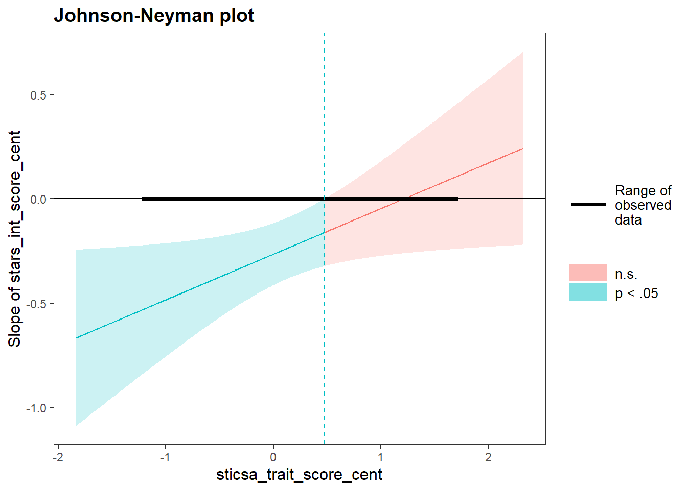
JOHNSON-NEYMAN INTERVAL 

When sticsa_trait_score_cent is OUTSIDE the interval [0.48, 13.58], the
slope of stars_int_score_cent is p < .05.

Note: The range of observed values of sticsa_trait_score_cent is [-1.21,
1.70]

SIMPLE SLOPES ANALYSIS 

Slope of stars_int_score_cent when sticsa_trait_score_cent = -0.60047717 (- 1 SD): 

   Est.   S.E.    2.5%   97.5%   t val.      p
------- ------ ------- ------- -------- ------
  -0.40   0.11   -0.60   -0.19    -3.75   0.00

Slope of stars_int_score_cent when sticsa_trait_score_cent =  0.02679718 (Mean): 

   Est.   S.E.    2.5%   97.5%   t val.      p
------- ------ ------- ------- -------- ------
  -0.26   0.08   -0.41   -0.11    -3.45   0.00

Slope of stars_int_score_cent when sticsa_trait_score_cent =  0.65407153 (+ 1 SD): 

   Est.   S.E.    2.5%   97.5%   t val.      p
------- ------ ------- ------- -------- ------
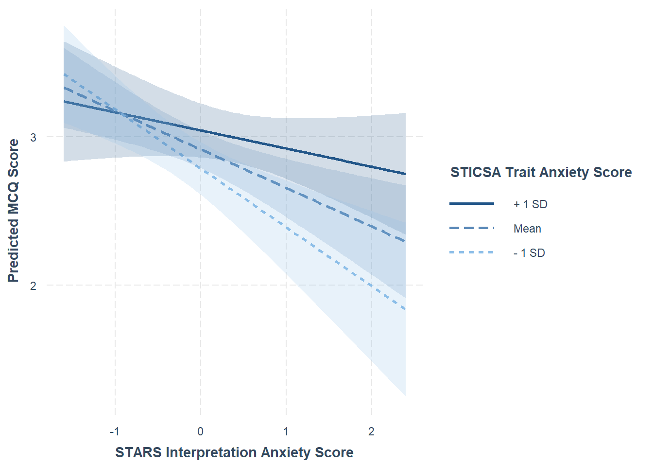
  -0.12   0.09   -0.30    0.06    -1.34   0.18

For a lovely visualisation of the simple slopes analysis, the interact_plot() function from the same package produces a beautiful plot with minimal effort. This plot output is also a ggplot object, so you can further add to or customise it from here if you prefer.

1interactions::interact_plot(
2  stars_mod_lm,
3  pred = stars_int_score_cent,
4  modx = sticsa_trait_score_cent,
5  interval = TRUE,
6  x.label = "STARS Interpretation Anxiety Score",
  y.label = "Predicted MCQ Score",
  legend.main = "STICSA Trait Anxiety Score"
  )

1: Produce a simple slopes interaction plot as follows:
2: Use the model stored in the object stars_mod_lm,
3: with the centered STARS Interpretation Anxiety score as the predictor,
4: and the centered STICSA Trait Anxiety score as the moderator,
5: with CIs included around the lines,
6: and custom labels for the x, y, and legend.

Well, that’s enough statistics for…well, to be honest, most of second year of UG! Aside from factor analysis and some other bits and pieces, we’ve covered a good portion of what you can expect your supervisees to have been taught previously.

From here, it would be a good idea to review the {discovr} tutorial in more depth for the specific analysis you’re thinking of using. However, at this point a lot of the content will be familiar - and you may even know a few tips and tricks that Andy doesn’t cover 🥳

Well done!

Overview

Setup

Packages

Data

Codebook

Categorical Predictors

Comparing Several Means

Plot

Fit the Model

Contrasts

Post-Hoc Tests

Factorial Designs

Fit the Model

Interaction Plot

EMMs

Simple Effects

Mixed Designs

Reshaping with pivot_*()

Fit the Model

Main Effects

Two-Way Interactions

Continuous Predictors

Mediation

Fit the Model

Results

Moderation

Centring

Fit the Model

Results

Reshaping with `pivot_*()`