library(tidyverse)03: Datasets
Overview
This tutorial is focused on working with datasets. It covers key functions and tips for reading in, viewing, and summarising datasets. It also introduces the pipe operator and a variety of common descriptive functions for investigating both whole datasets and individual variables, and concludes with a brief look at data visualisations with base R.
Setup
In the previous tutorial, we saw that there are three key steps to setting up to work in R:
- Create or open a project in RStudio
- Create or open a document to work in
- Load the necessary packages
Reading In
With a lot of the foundational skills of using R and RStudio in place, we’re ready to get stuck in working with datasets. For the purposes of practicing, we’re going to use some real, open-source data from a 2016 paper by Mealor et al. developing the Sussex Cognitive Styles Questionnaire (SCSQ). The SCSQ is a six-factor cognitive styles questionnaire validated by comparing responses from people with and without synaesthesia.
We’re going to start by importing, or “reading in”, the data from a location outside of R. The first job is to work out how that data is stored: the file format that it’s in, and the location we need to give to R to look for it.
File Types
For the purposes of these tutorials, we’ll primarily make use of .csv file types when reading in. CSV (Comma-Separated Values) is a common, program-agnostic file type without any fancy formatting, just plain text. To practice this, we’ll use the read_csv() function from the {readr} package (part of {tidyverse}).
One advantage of readr::read_csv() (as opposed to, say, the almost identically named base R package read.csv()) is that it will output a special kind of dataset, called a tibble. Tibbles are a fundamental component of {tidyverse}. They are a sort of embellished dataframe or table (“table” > “tbl” > “tibble”) with some extra bells and whistles for convenience. We’ll discover their features as we go, but you can get a quick overview of tibbles here.
Reading Other Filetypes
If you have data stored in other types of files, you may need other functions from other packages to read them in. It will depend substantially on what’s in the file and how the data are structured, so you will likely need to do some experimentation to find the best option.
Here are some possibilities to get you started. All of them (except the last) output a tibble.
- Excel (.xlsx):
readxl::read_xlsx() - SPSS (.sav):
haven::read_sav() - SAS (.sas):
haven::read_sas() - JSON:
rjson::fromJSON()
Our next job is to figure out where the data is stored. For the purposes of practice, we’ll look at two possibilities. First, that the data is stored in a local file on your computer; and second, that the data is hosted online somewhere, accessible via URL.
From File
The scenario you are most likely to encounter is that you have some data in a folder on your computer, and you’d like to read in this data to R so you can work with it. To practice this, in your Posit Cloud project there is a folder named “data” that contains a file called “syn_data.csv”. (If you are not on the Cloud, skip down to the next section.)
In order to use the read_csv() function, we need to give it the file path as a string (i.e. in "quotes"). Let’s make this easier by using a helper function: here::here().
What you should get is a string - a file path to the project you are currently in. On Posit Cloud, this will always be “/cloud/project” (unless you change it, which - don’t!). In any case, it will always point to the location of the .Rproj file that denotes your current project.
Why is this useful? Instead of having to write out long file paths (“C/Users/my_folder/What Was It called-again?/…”), or trying to figure out where your current file is relative to the data (or image, or whatever) that you are trying to find, here::here() uses the project file as a fixed point. So, all file paths can be written starting from the same point.
RepRoducibility: Reminder about paths
We talked about the issues that hard-coding absolute paths can cause in Tutorial 2.
The here::here() function generates the start of the file path, but likely (hopefully!) not all of your files are in the same folder. In our case, the project folder contains a data folder, which contains a file called syn_data.csv, which is the file we want to read in.
We can navigate there by adding more bits of the file path inside the brackets of the here::here() function, for example: here::here("this_folder/this_file.csv") will produce a file path to this_file.csv in the folder this_folder starting from the project folder.
From URL
If the data is hosted somewhere online, you can give the hosting URL to R as a string. Assuming you have an Internet connection (!), R will go to that URL and parse the data.
Codebook
RepRoducibility: Codebooks Make Data Readable
A codebook, also known as a data dictionary, is a document that describes the variables in a dataset. I strongly advise everyone to always share a codebook when uploading data online. Without a data dictionary, people who are not familiar with the data, won’t be able to understand what data represents and how to use it. I have found that data dictionaries also help me when I want to use data that I collected some months or years ago. Here is an example of what to include in a codebook.
To illustrate the importance of codebooks, have a look at syn_data by clicking on the object name in the environment and try to determine what information is stored in each variable.
The codebook below explains what the variables in this dataset represent.
| Variable Name | Type | Description |
|---|---|---|
| id_code | factor | Participant ID number |
| gender | factor | Participant gender, 0 = female, 1 = male |
| gc_score | numeric | Score on the grapheme-colour test of the Synesthesia Battery (Eagleman et al., 2007). Scores of 1.43 or lower indicate genuine synaesthesia (Rothen et al., 2013) |
| syn | factor | Whether the participant is a synaesthete (Yes) or not (No), regardless of type of synaesthesia |
| syn_graph_col | factor | Whether the participant has grapheme-colour synaethesia (Yes) or not (No) |
| syn_seq_space | factor | Whether the participant has sequence-space synaethesia (Yes) or not (No) |
| scsq_imagery | numeric | Mean score on the Imagery Abilitysubscale of the SCSQ |
| scsq_techspace | numeric | Mean score on the Technical/Spatial subscale of the SCSQ |
| scsq_language | numeric | Mean score on the Language and Word Forms subscale of the SCSQ |
| scsq_organise | numeric | Mean score on the Organisation subscale of the SCSQ |
| scsq_global | numeric | Mean score on the Global Bias subscale of the SCSQ |
| scsq_system | numeric | Mean score on the Systemising Tendency subscale of the SCSQ |
MoRe About: Synaesthesia
This dataset focuses on cognitive styles, particularly in people with and without a neuropsychological condition called synaesthesia. Synaesthesia is colloquially referred to as a “blending of the senses” that can manifest in many different ways. For example, some people with synaesthesia may perceive colours associated with letters or words, or see shapes when they hear music. These additional perceptions are typically automatic and consistent across time.
This particular study focused on two different types of synaesthesia: grapheme-colour and sequence-space. People with grapheme-colour synaesthesia experience colour associated with written language, i.e. graphemes. For instance, the letter “Q” may be purple, or the word “cactus” may be red (or a combination of colours).
People with sequence-space synaesthesia associate sequences, such as numbers, days of the week, or months of the year, with particular locations in physical space. For instance, Monday may be located up and to the right, or July near the left hip. Sequence-space synaesthetes can often precisely describe and point to the specific location of each element of the sequence.
There are also a variety of qualities associated with having synaesthesia of any type, so this dataset also includes a variable coding for having either (or both) types.
Viewing
We’ve now got some data to work with! Before we jump into doing anything with it, though, we should take a look at it. This is always a good idea to check that our data has read in correctly without any parsing errors. But in R our data is tucked away in an object, so how can we take a look at it?
Call the Object
Our first option is to call the object that contains our data. This is almost always an easy and straightforward way to get an instant look at what’s in our data.
As this object is a tibble, we can have a look at a few of those “bells and whistles” I mentioned earlier here.
- By default, tibbles like this one only print out up to the first ten rows at a time, and as many columns as conveniently fit in your current Source pane window size.
- You can scroll through this printout by clicking the numbers at the bottom (to move through rows) or the left and right arrows at the top (to scroll through columns).
- Each column has a little tag underneath it to tell you what kind of data is currently stored in it, for example
<dbl>for numeric/double and<chr>for character. - In the top left, the little box tells you what it is (“A tibble”) and the size of the dataset (“1211 x 12”).
Warning
There’s a big caveat here: calling an object to print it out works great with tibbles. For data stored in other formats, like matrices, there’s no preset formatting like this. If you accidentally call the name of an object that contains thousands of rows, R will try to print them all, which can lead to crashes. So, avoid calling very large objects directly like this if they aren’t tibbles.
A Glimpse of the Data
As mentioned above, just calling the dataset isn’t always super helpful - it depends on the size of your screen and even the width of your current window! As the next step, let’s get an overview of this dataset using the glimpse() function from the {dplyr} package.
This gives us a nice overview of all the variables we have in the data (each preceded by $, which we’ll come back to in the second half); what kind of data they are (e.g. <chr>, <dbl>, and so on); and a look at the first few values in each variable. This is a great way to check that all the variables you expect to be there are there, and that they contain (more or less) what you thought they should.
But what if we really want to get a look at the entire dataset? For that we need…
View Mode
We can have a look at the whole dataset more easily - and interact with it to some degree - by viewing it, which opens a copy of the dataset in the Source window to look through. We can do this with the View() function (note the capital “V”!).
This View mode has a few very handy features. Take a moment now to explore and work out how to do the following.
These features are really useful to have a quick poke around the data or check that everything is in order. However, keep in mind an important point: None of the changes made in View mode affect the data. View mode is essentially read-only; there’s no way to actually change the dataset or extract the values (like the range or max value) outside of copying them down by hand1. We’ll have to use R to work with the data in order to do that.
No Touching
If you are used to programs like SPSS or Excel, where you can directly edit or work with the data in the spreadsheet, switching to R can be quite a frustrating change. Even though View mode looks similar, it’s like the dataset is behind glass - you can’t affect it directly. As we start working with the data via objects and functions, it may feel a bit like you are trying to work blindfolded - you can’t actually “see” what you are doing as you do it.
If you feel that way, be reassured that it’s normal. Working with objects rather than with spreadsheets or data directly takes some getting used to, and it will get easier with practice. Use View() freely to check your work - I do!
Overall Summaries
We’ve now gained some confidence that our data looks like data should. We got a look at some summary information in View mode, but although this might have been useful for us in our initial checks, we can’t easily record or reproduce that information. Next, we’re going to look at some options for getting summary information about the whole dataset.
Basic Summary
The quickest and easiest check for a whole dataset is the base R function summary(). This function doesn’t do anything fancy (at all) but it does give you a very quick look at how all the variables have been read in, and an early indication if there’s anything exciting wonky going on.
Here, for example, notice the gender variable. This is intended to be a categorical variable, but clearly something has gone pear-shaped, because it has read in as a numeric variable. We have a related, but different issue with the syn_* variables, which also should be categorical (“Yes” and “No”), but instead have been read as numeric. Our other variables, gc_score and the scsq variables, should contain numeric information and it appears they do; for them, we get some helpful information and measures of central tendency.
We will ignore the categorical issue for now until we cover how to make changes to the dataset in a future tutorial.
summary() is quick, and because it’s a base-R function, it doesn’t need any package installations to work. However, it’s also of limited use: its output is ugly, and it would be pretty difficult to get any of those values out of that output for reporting!
Other Summaries
Besides the basic summary, there are many ready-made options in various packages to quickly produce summary tables. At the UG level, students are introduced datawizard::describe_distribution(), which is one such function. To use it, simply put the name of the dataset object inside the brackets.
Tip
Besides its default settings, the output can be further customised to add or remove particular statistics; see the help documentation.
The Pipe
Before we go on, we’re going to meet a new operator that will form the core of our coding style from this point onwards: the pipe. We’ll begin working with it a bit today, so let’s first explore why it’s so useful.
In this and the previous tutorial, we’ve seen some examples of “nested” code - functions nested within functions, as below.
round(mean(quiz_9am), digits = 2)To read this code, you have to start at the innermost level of nesting and work outwards. So, first R gets the quiz_9am object; then calculates the mean using mean(); then the output of mean() is the input to round(). For one or two levels of nesting, this is still legible, but can quickly become very difficult for humans to track.
One solution is to use the pipe operator, |>. The pipe “chains” commands one after the other by taking the output of the preceding command and “piping it into” the next command, allowing a much more natural and readable sequence of steps - sequentially, rather than nested. The pipe version of the above might look like this:
quiz_9am |>
  mean() |>
  round(digits = 2)
This style maps on a lot more naturally to how we would read or understand the steps in this command in natural language.
Definition: The Pipe Operator
The pipe operator, |>, takes the output of the code on its left-hand side (LHS) and passes it, by default, into the first unnamed argument of its right-hand side (RHS)2. Many functions - both from the {tidyverse} and not - are already set up so that the first argument is the data, and {tidyverse} functions are explicitly designed this way in order to work best with the pipe.
The pipe operator may appear in two formats.
- The native pipe, |>. This is the pipe we will use throughout these tutorials. It is called the “native” pipe because it is inbuilt into R and doesn’t require any specific package to use.
- The {magrittr} pipe, %>%. This pipe comes from {tidyverse}, and in particular requires the {magrittr} package to use. You will very commonly see this pipe in scripts, Stack Overflow posts, from ChatGPT, etc. as until the native pipe was introduced to R in 2022, the {magrittr} pipe was “the pipe” for R.
In most cases, including almost all of the code we will learn in these tutorials, the two pipes are interchangeable and will result in the same output.
In cases where you would like the output of the pipe to go someplace other than the first unnamed argument, you can determine where the piped-in information should go using a “placeholder”. The most noticeable difference between the native vs magrittr pipes is that they have different placeholders. The native pipe (|>) uses underscore _ as its placeholder, while the magrittr pipe (%>%) uses the dot/full stop .. There’s an example using placeholders below to help make this clearer.
From this point forward, we’ll start working with the native pipe. The following sections will have specific examples on using the pipe to practice. Working with the pipe is also a good chance to practice “translating” R code into English, which we’ll do as we go. To give you an idea, here’s an example of how we can read the following code. We’ll typically read |> as “and then”, taking the output of whatever the preceding line produces and passing it on to the next line.
- 1
-
Create a new object,
some_numbers, that contains a vector of some numbers. - 2
-
Take
some_numbers, and then… - 3
- Calculate the mean of those numbers, and then…
- 4
- Round that mean to two decimal places, which outputs:
[1] 6.37It might seem strange that the mean() and round() functions appear to be “empty”. Take the third step above, which just reads mean(). There’s nothing in the brackets, so it appears that the mean() function is working on nothing! However, remember that the pipe passes its LHS to the first unnamed argument of its RHS3. In this example, the object some_numbers is the input on the LHS, which is being “piped into” the first unnamed argument of the mean() function on the RHS, which is x, the data or values to work with, as we saw last week. We don’t have to explicitly specify this; it’s just how the pipe works by default.
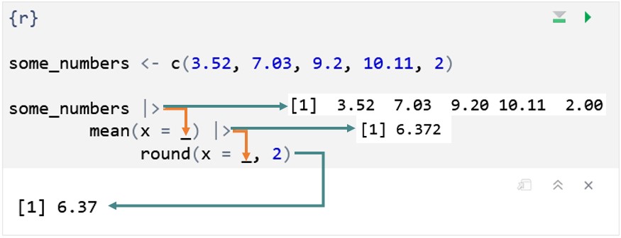
To illustrate this more clearly, here’s the same code explicitly including the placeholders to indicate where the piped-in information goes:
some_numbers <- c(3.52, 7.03, 9.2, 10.11, 2)

some_numbers |>
  mean(x = _) |>
  round(x = _, 2)
Think of the placeholder like a bucket or landing pad, where the information coming in from the pipe falls. In this example, the placeholders aren’t necessary, because at each step, we already want the piped-in information to go into the first argument, which we have left unnamed, and which is conveniently, in both cases, x, the data or values to work with; but including the placeholders (and, necessarily if we want to use placeholders, the argument names) helps to see what’s going on.
MoRe About: Placeholders and Named Arguments
A minor point here, but one that can cause issues especially if you want to adapt code using different pipes: If you want to use the _ placeholder with the native pipe |>, you must name the argument. The . placeholder for the magrittr pipe %>% doesn’t have this requirement:
some_numbers |>
  mean(_)
Error: pipe placeholder can only be used as a named argument (<text>:2:3)some_numbers %>%
mean(.)[1] 6.372To make the pipe operation fully explicit, the image below shows the progress of information through the same pipe. The orange arrows show how the piped-in information is passed from one function to the next. The teal arrows show what is produced at each step of the pipe - which is what is passed on to the next function via the orange arrows/pipe.
MoRe About: The Logic of Piping
Imagine we wanted to bake a Victoria sponge cake using R. Translating the steps into R, we might get something like this:
ingredients |>
  mix(order = c("wet", "dry")) |>
  pour(shape = "round", number = 2, lining = TRUE) |>
  bake(temp = 190, time = 20) |>
  cool() |>
  assemble(filling = c("buttercream", "jam"), topping = "icing_sugar") |>
  devour()
At each step, |> takes whatever the previous step produces and passes it on to the next step. So, we begin with ingredients - presumably an object that contains our flour, sugar, eggs, etc - which is “piped into” the mix() function. The output of that function might be all our ingredients mixed together in a bowl, which is then piped into the pour() function, and so on.
Notice for example, the function cool(), which doesn’t appear to have anything in it. It actually does: the cool() function would work with whatever the output of the bake() function was above it: a freshly baked cake straight out of the oven.
Without the pipe, our command might look something like this, which must be read from the inside out rather from top to bottom:
devour(
  assemble(
      cool(
        bake(
          pour(
            mix(ingredients,
                order = c("wet", "dry")),
            shape = "round", number = 2, lining = TRUE),
          temp = 190, time = 20)
      ),
    filling = c("buttercream", "jam"), topping = "icing_sugar"
  )
)
This is, I am sure you will agree, as absolutely horrifying as a soggy bottom on a cake.
RepRoducibility: Base R or Packages?
To make code more reproducible, it is a good idea to use base R instead of an additional package whenever possible. In most cases %>% and |> will be able to achieve the same goal, so it is a good idea to use |> unless you need to make use of some specific functionality of %>%.
Describing Datasets
To start, we’ll work again with the whole dataset and look at some helpful functions that are often important for validating our data processing.
nrow(): Returns the number of rows as a numeric value.ncol(): Returns the number of columns as a numeric value.names(): Returns a character vector of the names of the columns of a dataset (and also the names of elements for other types of input).
If your dataset is structured like this one is - with a single participant per row - then nrow() is a common stand-in for counting participants.
Using the native pipe, we can print out the number of columns and the names of those columns in the syn_data dataset:
syn_data |>
  ncol()
[1] 12syn_data |>
names() [1] "id_code" "gender" "gc_score" "syn"
[5] "syn_graph_col" "syn_seq_space" "scsq_imagery" "scsq_techspace"
[9] "scsq_language" "scsq_organise" "scsq_global" "scsq_system" The new line after the pipe isn’t essential (it will run exactly the same way) but it is highly recommended. Although it doesn’t make much of a difference here, we will shortly get to longer commands where the new line for each new function will make a big difference to legibility.
MoRe About: Reading the Pipe
If a command like syn_data |> names() looks a bit strange, let’s take a closer look at it.
This command is equivalent to names(syn_data), which might look a bit more familiar based on what we’ve done so far. The pipe takes whatever comes before it - in this case, the dataset syn_data - and pipes it into the first argument of the function that comes after it. The names() function only accepts one object as input, so syn_data is passed to names() as that single object. It looks like the names() function is empty, because there’s nothing in the brackets, but that’s because the dataset is being “piped in” from above.
We can make this a bit more explicit using the placeholder:
syn_data |>
  names(x = _)
[1] "id_code" "gender" "gc_score" "syn"
[5] "syn_graph_col" "syn_seq_space" "scsq_imagery" "scsq_techspace"
[9] "scsq_language" "scsq_organise" "scsq_global" "scsq_system" The underscore is the “placeholder” for the native pipe; in other words, it explicitly indicates where the object should be placed that is being piped in, like a “bucket” that catches whatever comes out of the pipe! This makes it a bit clearer to see that the object syn_data is going into the names() function, and specifically the x argument.
Describing Variables
Once we’ve had a look at the whole dataset, it’s time to drill down into individual variables. We may want to calculate quick descriptives or investigate what’s going on with particular variables that seem to have issues.
To do this, we’ll start working quite a bit with the {dplyr} package. {dplyr} is a core part of the {tidyverse}, and the package generally is focused on user-friendly and easily readable tools for data manipulation. The essential {dplyr} functions will form a core part of the next few weeks when we really get into to working with data.
Counting
We’ll start by having a look at character or categorical variables. Here we’ll meet a new {dplyr} function: dplyr::count(). This function is a friendly way to obtain (as you might expect!) counts of the number of times each unique value appears in a variable. As with just about everything in {dplyr}, it takes a tibble as input and produces a tibble as output.
Using the pipe structure we’ve seen previously, the general form is:
dataset_name |>
  dplyr::count(variable_to_count, optionally_another, ...)
Minimally you need to provide a single variable to count the values in, but you can add more, separated by commas, to further subdivide the counts.
For example, if we wanted to count the number of grapheme-colour synaesthetes in this dataset, we could use the count() function as follows:
syn_data |>
  dplyr::count(syn_graph_col)
As you can see, the output from this function is a new summary tibble containing only the unique values in each variable, and a count, in the new “n” variable, of how many times that value (or combination of values) appeared.
Note that this does not change or add anything to your original dataset! Instead, this function creates a brand-new tibble with the requested information.
MoRe About: Reading the Pipe
If you feel like you’re good with the pipe, you can skip this - but if you’re wondering about the command above, this explains a bit more, as this code structure is going to come up again and again as we work with different data wrangling functions.
If we have a look at the help documentation for the dplyr::count() function, we can see in the Usage section that it takes the form:
count(
  x,
  ...
  )
We also see in the Arguments section that x is a “data frame, data frame extension (e.g. a tibble)”, and ... is “Variables to group by”.
Taking another look at the command we wrote above:
syn_data |>
  dplyr::count(syn_graph_col)
We can see that syn_graph_col is the name of the variable in syn_data that we wanted to count the values within. But where has syn_data itself gone?
If we make this explicit, we could write the same command as follows:
syn_data |>
  dplyr::count(
    x = _,
    syn_graph_col)
This makes it clear that the tibble syn_data coming in from the pipe is landing in the x argument. Remember that the information piped in goes by default into the first unnamed argument. The first argument of dplyr::count() is x, which should be the dataset to work with. Because this is exactly where we wanted the dataset to go, we can just leave out the x argument altogether - that is, by leaving it unnamed, and because it is first, the dataset is piped into that argument by default.
The resulting command:
syn_data |>
  dplyr::count(syn_graph_col)
is not only fairly simple and easy to parse, but maps on nicely to actual human language, which might be something like:
Take the
syn_datadataset and then count the values in thesyn_graph_colvariable.
Subsetting
To work with individual variables, we need to get them out of the dataset. Specifically, for many of the functions we’re about to use, we will need the values stored in those variables as vectors. We can do this in two ways: $ notation, or the function dplyr::pull()4.
Subsetting with $ is the base-R method, and it takes the general form:
dataset_name$variable_to_subsetSubsetting with dplyr::pull() is a {tidyverse} method of accomplishing the same thing. Using the pipe structure we’ve seen previously, the general form is:
dataset_name |>
  dplyr::pull(variable_to_subset)
For example, let’s get out all of the values in the scsq_global variable using each method. (To keep this tutorial legible, I’ve only printed out the first 10 values.)
## Base-R $ subsetting
syn_data$scsq_global
[1] 1.50 1.13 2.13 2.25 2.50 4.13 3.00 2.50 3.88 1.88
[ reached getOption("max.print") -- omitted 1201 entries ]## dplyr::pull subsetting
syn_data |>
dplyr::pull(scsq_global) [1] 1.50 1.13 2.13 2.25 2.50 4.13 3.00 2.50 3.88 1.88
[ reached getOption("max.print") -- omitted 1201 entries ]If you’re wondering when to use $ and when to use dplyr::pull(), the answer depends on what you want to do! We’ll see some examples of both in just a moment.
Descriptives
Next up, we can start doing some calculations with these values. The base-R {stats} package contains a wide variety of very sensibly-named functions that calculate common descriptive statistics, which we also briefly encountered in the previous tutorial. As a reminder, these include:
mean()andmedian()(there is a functionmode(), but it doesn’t do what we’d like it to here!)min()for minimum value,max()for maximum valuerange()for both minimum and maximum value in a single vectorsd()for standard deviation
As a reminder, a key feature of all of these functions is that, by default, they return NA if there are any NAs (missing values) present. So, they all have an argument, na.rm =, which determines whether NAs should be removed. By default this argument is set to FALSE (NAs should NOT be removed), but if you want to get the calculation ignoring any NAs, you can set this argument to TRUE instead.
Let’s look some more at the scsq_global variable. Now that we know how to subset it from the dataset - producing a vector of numbers - we can use the functions above to calculate some information. Let’s get the mean and the standard deviation, using each subsetting method once.
mean(syn_data$scsq_global, na.rm = TRUE)[1] 2.939389syn_data |>
dplyr::pull(scsq_global) |>
sd(na.rm = TRUE)[1] 0.6011931As a quick check to get an individual number, this method is quite useful. However, you may have noticed that if we wanted this information for lots of variables, this would be repetitive, laborious, and prone to error. We’ve already seen how to use existing summary functions, but we will also look at creating custom summary tables in a future tutorial.
Visualisations
The final piece we will look at today will be base-R data visualisations in the {graphics} package. These built-in graphics functions are particularly helpful for quick spot checks during data cleaning and manipulation. For high-quality, fully customisable, professional data visualisations, we will use the {ggplot2} package, covered in depth later on in this course.
To get the idea, there are a few options for common plots:
hist()for histogramsboxplot()andbarplot()plot()for scatterplots
As one example, let’s look at the hist() function to create a histogram. The help documentation lists a large number of possible arguments to tweak the appearance of the histogram, but unless you’re quite keen, I wouldn’t worry about them too much, since we’ll be building our own high-quality custom data visualisations in a few weeks. For now, we’ll just look at three:
main, to give the plot a titlexlabandylab, to label the x and y axes respectively.
So, both with and without the labelling, we get:
hist(syn_data$scsq_global)
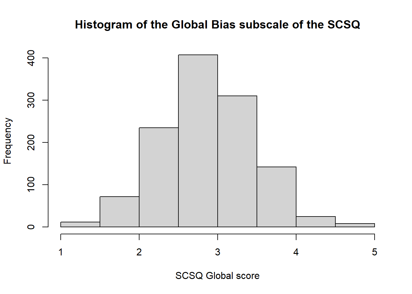
hist(syn_data$scsq_global,
main = "Histogram of the Global Bias subscale of the SCSQ",
xlab = "SCSQ Global score")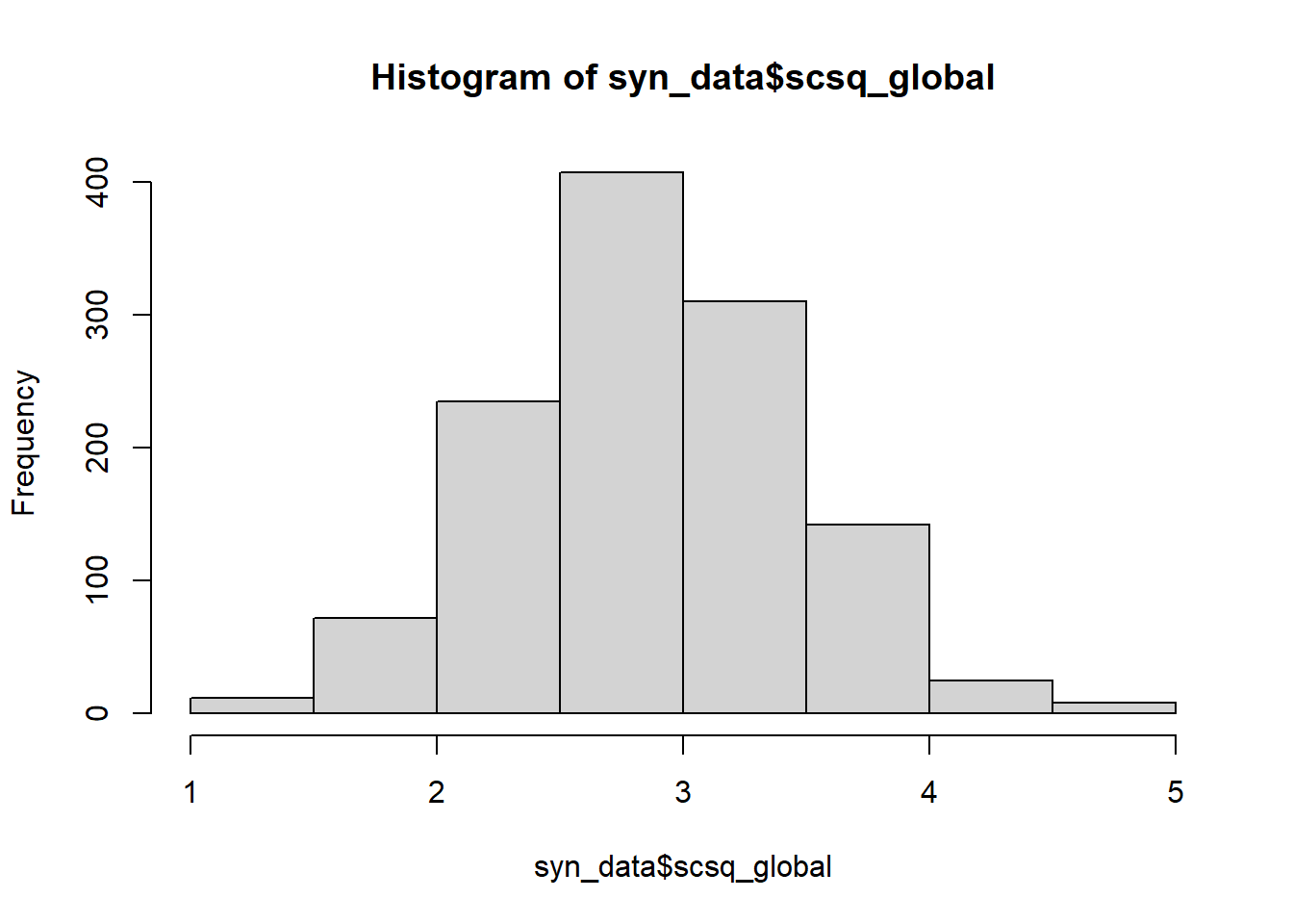
For more help and examples with base R graphics, try this quick guide.
Exercises
The following exercises will help you practice the new functions and techniques in the second half of this tutorial. Have a go at each, using the solutions if you get stuck. Good luck!
Exercise
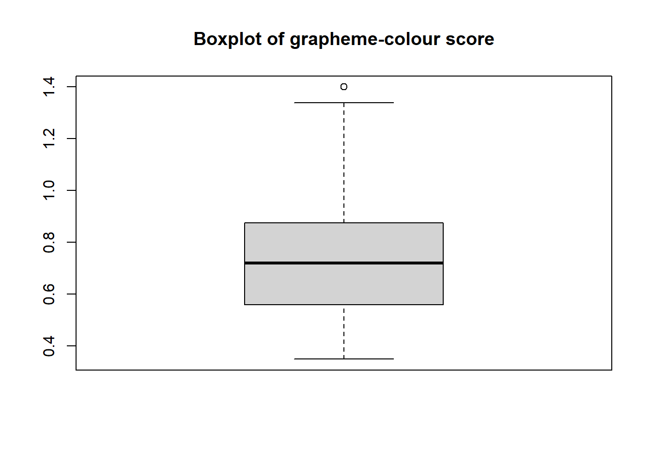
Try making a boxplot of the gc_score variable. Use either $ or pull() as you like.
Optionally, if you feel so inclined, use the help documentation to spruce up your plot a bit, such as changing the title label.
Solution
syn_data |>
dplyr::pull(gc_score) |>
boxplot()
syn_data |>
dplyr::pull(gc_score) |>
boxplot(
main = "Boxplot of grapheme-colour score")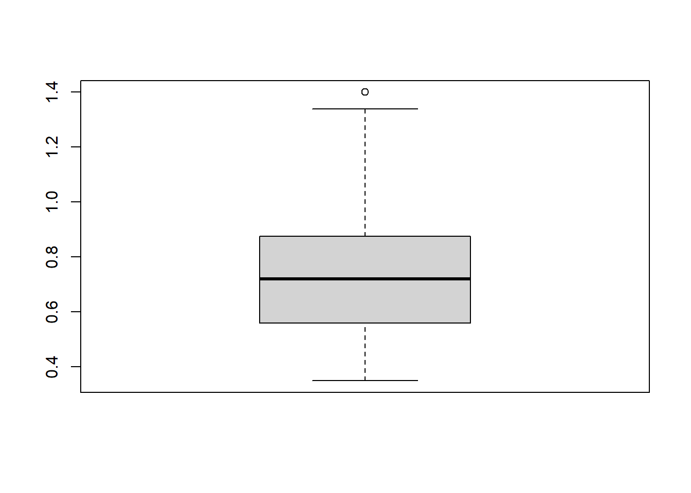
Exercise
CHALLENGE: Try making a barplot and a scatterplot.
For the barplot, make a visualisation of how many people are synaesthetes or not (regardless of synaesthesia type).
For the scatterplot, choose any two SCSQ measures.
Both of these require some creative problem-solving using the help documentation and the skills and functions covered in this tutorial.
Solution
The following solutions are options - if you found another way to make the same or similar plots, well done!
Barplots require two sets of values: a categorical one on the horizontal x axis and a continuous one on the vertical y axis. For something like frequency counts, then, we have to first do the counting, then pass those counts onto barplot(). Luckily we already know how to count categorical variables.
The help documentation is most helpful in the Examples section, where it shows actual examples of how the function works. There we can see an example of the formula method, y ~ x, which I’ve used below. Since we’re piping in the data to an argument that is not the first, I’ve used the placeholder in the data = _ argument to finish the command.
syn_data |>
dplyr::count(syn) |>
barplot(
n ~ syn,
data = _)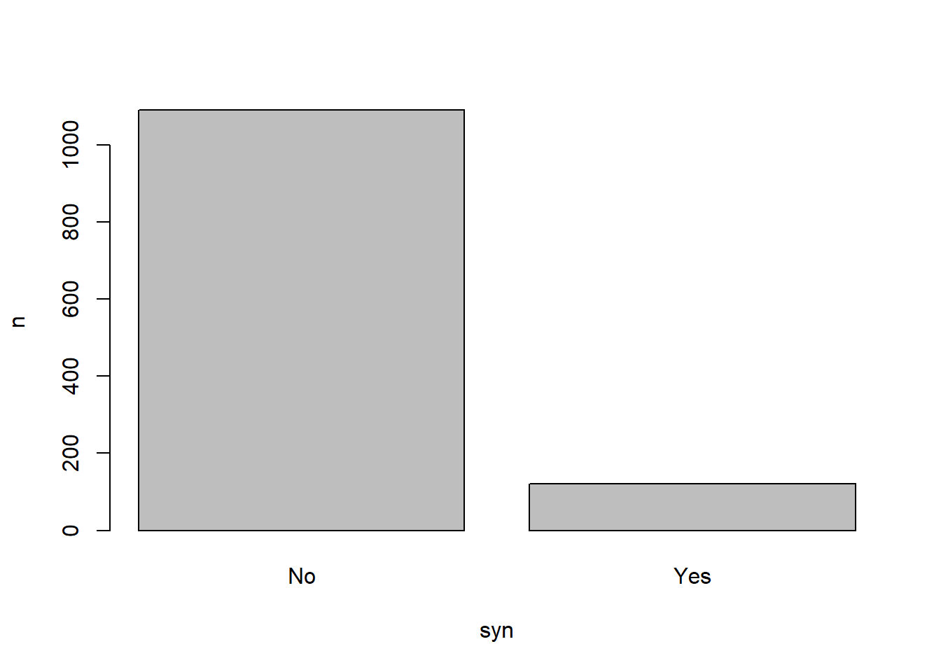
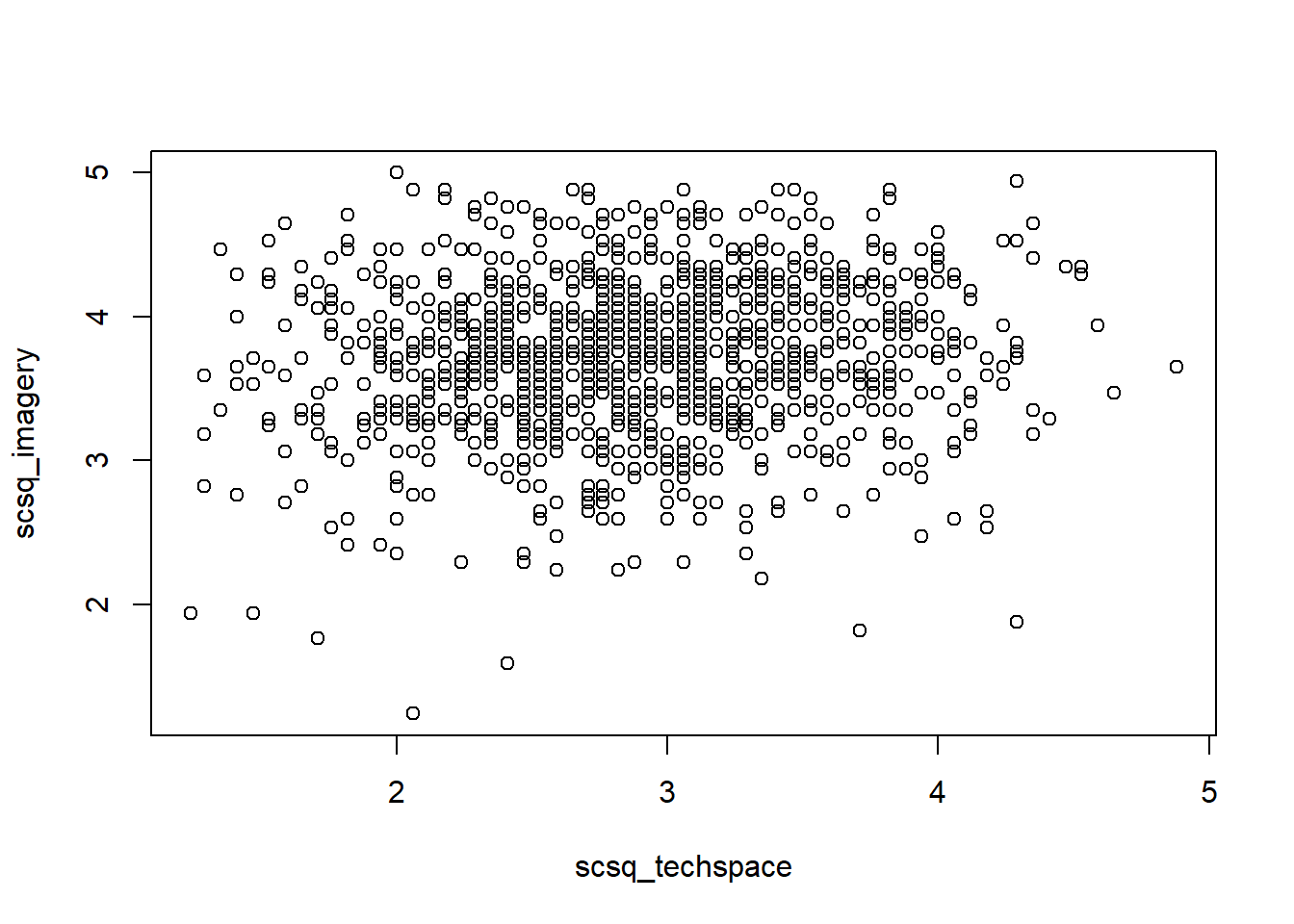
For the scatterplot, there are a couple of options. We can either supply x and y separately using $ subsetting, or use the same y ~ x formula we saw for barplots previously.
## Using subsetting
plot(syn_data$scsq_techspace, syn_data$scsq_imagery)
## Using a formula
syn_data |>
  plot(scsq_imagery ~ scsq_techspace, data = _)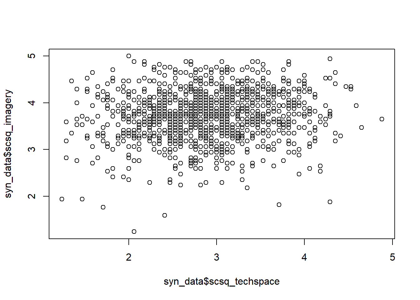
Footnotes
Remember last week I mentioned that “first unnamed arguments” would be important? Here’s why! Look back on 02 IntRoductions if you’d like a refresher.↩︎
I’m intentionally using this slightly obtuse terminology because it often appears in help documentation, so it’s worth getting used to these acronyms.↩︎
This function always makes me think of one of those arcade claw machines reaching into the dataset to grab the values you want.↩︎
You can call this object anything you like; I use “px” as shorthand for “participant.”↩︎
