library(dplyr)
## OR
library(tidyverse)

library(GGally)
library(correlation)
library(kableExtra)06: Mutate and Summarise
Overview
This tutorial covers three more essential {dplyr} functions: workhorses mutate() and summarise(), and helper group_by().
Very similar in structure, the first two functions primarily differ in output. mutate() makes changes within a given dataset by creating new variables (columns) whereas summarise() uses the information in a given dataset to create a new, separate summary dataset.
The last, group_by(), is a helper function that allows new variables or summaries to be created within subgroups.
Setup
Packages
We will again be focusing on {dplyr} today, which contains all three of our main functions. You can either load {dplyr} alone, or all of {tidyverse} - it won’t make a difference, but you only need one or the other.
We’ll also need {GGally} for correlograms, {correlation} for, well, I’ll give you three guesses!, and {kableExtra} for table formatting.
Data
Today we’re continuing to work with the same dataset as last week. Courtesy of fantastic Sussex colleague Jenny Terry, this dataset contains real data about statistics and maths anxiety.
Codebook
There’s quite a bit in this dataset, so you will need to refer to the codebook below for a description of all the variables.
Dataset Info Recap
This study explored the difference between maths and statistics anxiety, widely assumed to be different constructs. Participants completed the Statistics Anxiety Rating Scale (STARS) and Maths Anxiety Rating Scale - Revised (R-MARS), as well as modified versions, the STARS-M and R-MARS-S. In the modified versions of the scales, references to statistics and maths were swapped; for example, the STARS item “Studying for an examination in a statistics course” became the STARS-M item “Studying for an examination in a maths course”; and the R-MARS item “Walking into a maths class” because the R-MARS-S item “Walking into a statistics class”.
Participants also completed the State-Trait Inventory for Cognitive and Somatic Anxiety (STICSA). They completed the state anxiety items twice: once before, and once after, answering a set of five MCQ questions. These MCQ questions were either about maths, or about statistics; each participant only saw one of the two MCQ conditions.
Important
For learning purposes, I’ve randomly generated some additional variables to add to the dataset containing info on distribution channel, consent, gender, and age. Especially for the consent variable, don’t worry: all the participants in this dataset did consent to the original study. I’ve simulated and added this variable in later to practice removing participants.
| Variable | Type | Description |
|---|---|---|
| id | Categorical | Unique ID code |
| distribution | Categorical | Channel through which the study was completed, either "preview" or "anonymous" (the latter representing "real" data). Note that this variable has been randomly generated and does NOT reflect genuine responses. |
| consent | Categorical | Whether the participant read and consented to participate ("Yes") or not ("No"). Note that this variable has been randomly generated and does NOT reflect genuine responses; all participants in this dataset did originally consent to participate. |
| gender | Categorical | Gender identity, one of "female", "male", "non-binary", or "other/pnts". "pnts" is an abbreviation for "Prefer not to say". Note that this variable has been randomly generated and does NOT reflect genuine responses. |
| age | Numeric | Age in years. Note that this variable has been randomly generated and does NOT reflect genuine responses. |
| mcq | Categorical | Independent variable for MCQ question condition, whether the participant saw MCQ questions about mathematics ("maths") or statistics ("stats"). |
| stars_[sub][number] | Numeric | Item on the Statistics Anxiety Rating Scale. There are three subscales, denoted with [sub] in the name: - [test]: Test anxiety - [help]: Asking for Help - [int]: Interpretation Anxiety. [num] corresponds to the item number. Responses given on a Likert scale from 1 (no anxiety) to 5 (a great deal of anxiety), so higher scores reflect higher levels of anxiety. |
| stars_m_[sub][number] | Numeric | Item on the Statistics Anxiety Rating Scale - Maths, a modified version of the STARS with all references to statistics replaced with maths. There are three subscales, denoted with [sub] in the name: - [test]: Test anxiety - [help]: Asking for Help - [int]: Interpretation Anxiety. [num] corresponds to the item number. Responses given on a Likert scale from 1 (no anxiety) to 5 (a great deal of anxiety), so higher scores reflect higher levels of anxiety. |
| rmars_[sub][number] | Numeric | Item on the Revised Maths Anxiety Rating Scale. There are three subscales, denoted with [sub] in the name: - [test]: Test anxiety - [num]: Numerical Task Anxiety - [course]: Course anxiety. [num] corresponds to the item number. Responses given on a Likert scale from 1 (not at all) to 5 (very much), so higher scores reflect higher levels of anxiety. |
| rmars_s_[sub][number] | Numeric | Item on the Revised Maths Anxiety Rating Scale - Statistics, a modified version of the MARS with all references to maths replaced with statistics. There are three subscales, denoted with [sub] in the name: - [test]: Test anxiety - [num]: Numerical Task Anxiety - [course]: Course anxiety. [num] corresponds to the item number. Responses given on a Likert scale from 1 (not at all) to 5 (very much), so higher scores reflect higher levels of anxiety. |
| sticsa_trait_[number] | Numeric | Item on the State-Trait Inventory for Cognitive and Somatic Anxiety, Trait subscale. [num] corresponds to the item number. Responses given on a Likert scale from 1 (not at all) to 4 (very much so), so higher scores reflect higher levels of anxiety. |
| sticsa_[time]_state_[number] | Numeric | Item on the State-Trait Inventory for Cognitive and Somatic Anxiety, State subscale. [time] denotes one of two times of administration: before completing the MCQ task ("pre"), or after ("post"). [num] corresponds to the item number. Responses given on a Likert scale from 1 (not at all) to 4 (very much so), so higher scores reflect higher levels of anxiety. |
| mcq_stats_[num] | Categorical | Correct (1) or incorrect (0) response to MCQ questions about statistics, covering mean ([number] = 1), standard deviation (2), confidence intervals (3), beta coefficient (4), and standard error (5). |
| mcq_maths_[num] | Categorical | Correct (1) or incorrect (0) response to MCQ questions about maths, covering mean ([number] = 1), standard deviation (2), confidence intervals (3), beta coefficient (4), and standard error (5). |
Mutate
The mutate() function is one of the most essential functions from the {dplyr} package. Its primary job is to easily and transparently make changes within a dataset - in particular, a tibble.
General Format
To make a single, straightforward change to a tibble, use the general format:
dataset_name |>
  dplyr::mutate(
    variable_name = instructions_for_creating_the_variable
  )
variable_name is the name of the variable that will be changed by mutate(). This can be any name that follows R’s object naming rules. There are two main options for this name:
- If the dataset does not already contain a variable called
variable_name, a new variable will be added to the dataset. - If the dataset does already contain a variable called
variable_name, the new variable will silently1 replace (i.e. overwrite) the existing variable with the same name.
instructions_for_creating_the_variable tells the function how to create variable_name. These instructions can be any valid R code, from a single value or constant, to complicated calculations or combinations of other variables. You can think of these instructions exactly the same way as the vector calculations we covered earlier, and they must return a series of values that is the same length as the existing dataset.
Tip
Although creating or modifying variables will likely be the most frequent way you use mutate(), it has other handy features such as:
- Deleting variables
- Deciding where newly created variables appear in the dataset
- Deciding which variables appear in the output, depending on which you’ve used
See the help documentation for more by running help(mutate) or ?mutate in the Console.
Adding and Changing Variables
Let’s have a look at how these two operations work in mutate().
First, let’s see how to add new variables. Imagine we have found some collaborators to work with and we want to combine our datasets. To keep track of where the data came from, we want to add a lab variable at the start of our existing dataset containing the name of the university before we add more data.
- 1
- Take the dataset and make the following changes:
- 2
-
Create a new variable,
lab, that contains the value"Sussex" - 3
- Put this variable before the first variable in the existing dataset.
Error Watch: Vector Size
Note that in this case, I’ve given a single value, "Sussex", as the content of the new variable. R will “recycle” this single value across all of the rows to create a constant. However, if I tried to do this with a longer vector, I’ll get an error:
anx_data |>
  dplyr::mutate(
    lab = c("Sussex", "Glasgow"),
    .before = 1
  )
Error in `dplyr::mutate()`:
ℹ In argument: `lab = c("Sussex", "Glasgow")`.
Caused by error:
! `lab` must be size 465 or 1, not 2.In this case I might need rep() (for creating vectors of repeating values), sample() (for creating random subsamples), or another helper function to generate the vector to add.
Next, let’s look at changing existing variables. For example, I know that gender and mcq are meant to be factors (also called “categorical data” in SPSS and elsewhere). So, let’s convert each of these two variables into factor data type.
For ease of reading the output, I’m using the .keep = "used" argument, which only outputs variables that have been used in the preceding operation. This is for demonstration purposes and is great for checking your changes are correct, but make sure you remove this argument if you use this code yourself.
1anx_data |>
  dplyr::mutate(
2    gender = factor(gender),
    mcq = factor(mcq),
    ## OMIT this line for real analysis
3    .keep = "used"
)- 1
- Take the dataset and make the following changes:
- 2
-
For the
genderandmcqvariables, convert the existing variable into a factor and then replace the existing variable with the new one. - 3
- Only output the variables that were used or created in this operation.
Finally, once I’ve checked the code works by examining the output, if I want to actually change my dataset, I have to assign the output of these commands to the dataset.
What is reverse-coding?
In many multi-item measures, some items are reversed in the way that they capture a particular construct. In this particular example, items on the STICSA are worded so that a higher numerical response (closer to the “very much so” end of the scale) indicates more anxiety, such as item 4: “I think that others won’t approve of me”.
However, reverse-coded items are intended to capture the same ideas, but in reverse. A reversed version of item 17 might read, “I can concentrate easily with no intrusive thoughts.” In this case, a higher numerical response (closer to the “very much so” end of the scale) would indicate less anxiety. In order for these reversed items to be aligned with the other items on the scale, so that together they form a cohesive score, the coding of the response scale must be flipped: high becomes low, and low becomes high.
If the response scale is a numerical integer sequence, as this one is, then the simplest way to reverse-code the responses is to subtract every response from the maximum possible response plus one. Here, the STICSA response scale is from 1 to 4; the maximum possible response is 4, plus one is 5. So, to reverse-code the responses, we need to subtract each rating on this item from 5. A high score (4) will be become a low score (5 - 4 = 1), and vice versa for a low score (5 - 1 = 4).
Composite Scores
Row-wise magic is good magic. - Hadley Wickham
A very common mutate() task is to create a composite score from multiple variables - for example, an overall trait anxiety score from our sticsa_trait items. Let’s create an overall score that contains the mean of the ratings2 on each of the STICSA trait anxiety items, for each participant.
To do this, we need two new functions.
The first new function,
dplyr::c_across(), provides an efficient way to select multiple variables to contribute to the calculation - namely, by using<tidyselect>semantics.The second new function is actually a pair of functions,
dplyr::rowwise()anddplyr::ungroup(). These two respectively impose and remove an internal structure to the dataset, such that each row is treated like its own group, and any operations are done within those row-wise groups.
Let’s see the combination of these two in action.
Important
The code below assumes a dataset structured so there is information from each participant on only and exactly one row in the dataset.
If your data has observations from the same participants on multiple rows, you will need to reshape your data or otherwise adapt the code to suit your data structure.
1anx_data <- anx_data |>
2  dplyr::rowwise() |>
3  dplyr::mutate(
    sticsa_trait_score = mean(c_across(starts_with("sticsa_trait")),
                        na.rm = TRUE)
  ) |>
4 dplyr::ungroup()- 1
-
Overwrite the
anx_datadataset with the following output: take the existinganx_datadataset, and then - 2
- Group the dataset by row, so any subsequent calculations will be done for each row separately, and then
- 3
-
Create the new
sticsa_trait_scorevariable by taking the mean of all the values in variables that start with the string “sticsa_trait” (ignoring any missing values), and then - 4
-
Remove the by-row grouping that was created by
rowwise()to output an ungrouped dataset.
Tip
For lots more details and examples on rowwise() and rowwise operations with {dplyr} - including which other scenarios in which a row-wise dataset would be useful - run vignette("rowwise") in the Console.
Conditionals
There are many functions out there for recoding variables (let’s wave cheerfully at dplyr::recode() as we fly by it without stopping), but the following method, using dplyr::case_when(), is recommended because it is so versatile. It can be used to recode the values from one variable into new one, but it can also combine information across variables and handle multiple conditionals. It essentially allows a series of if-else statements without having to actually have lots of if-else statements.
The generic format of dplyr::case_when() can be stated as follows:
dataset_name |>
  dplyr::mutate(
    new_variable = dplyr::case_when(
      logical_assertion ~ value,
      logical_assertion ~ value,
      .default = value_to_use_for_cases_with_no_matches
    )
  )
logical_assertion is any R code that returns TRUE and FALSE values. These should be very familiar by now!
value is the value to assign to new_variable for the cases for which logical_assertion returns TRUE.
The assertions are evaluated sequentially (from first to last in the order they are written in the function), and the first match determines the value. This means that the assertions must be ordered from most specific to least specific.
Testing Assertions
The assertions for dplyr::case_when() are the same as the ones we used previously in dplyr::filter(). In fact, if you need to test the assertion you are writing to ensure that your code will work as you want, you can try the same assertion in dplyr::filter() to check whether the cases it returns are only and exactly the ones you want to change.
Let’s look at two examples of how dplyr::case_when() might come in handy.
One-Variable Input
We’ve created our composite sticsa_trait_score variable previously, and now we may want to change this continuous score into a categorical variable indicating whether or not participants display clinical levels of anxiety. So, we can use case_when() to recode sticsa_trait_score into a new sticsa_trait_cat variable.
1anxiety_cutoff <- 2.047619

2anx_data <- anx_data |>
3  dplyr::mutate(
4    sticsa_trait_cat = dplyr::case_when(
5      sticsa_trait_score >= anxiety_cutoff ~ "clinical",
6      sticsa_trait_score < anxiety_cutoff ~ "non-clinical",
7      .default = NA
    )
)- 1
-
Create a new object,
anxiety_cutoff, containing the threshold value for separating clinical from non-clinical anxiety. This one is from Van Dam et al., 2013. - 2
-
Overwrite the
anx_dataobject by taking the dataset, and then… - 3
- Making a change to it by…
- 4
-
Creating a new variable,
anxiety_cat, by applying the following rules: - 5
-
For cases where the value of
sticsa_trait_scoreis greater than or equal toanxiety_cutoff, assign the value “clinical” tosticsa_trait_cat - 6
-
For cases where the value of
sticsa_trait_scoreis less thananxiety_cutoff, assign the value “non-clinical” tosticsa_trait_cat - 7
-
For cases that don’t match any of the preceding criteria, assign
NAtosticsa_trait_cat
Why the new
anxiety_cutoff object?
In the code above, the cutoff value is stored in a new object, anxiety_cutoff, which is then used in the subsequent case_when() conditions. Why take this extra step?
This is a matter of style, since the output of this code would be entirely identical if I wrote the cutoff value into the case_when() assertions directly (e.g. sticsa_trait_score >= 2.047619). I have done it this way for a few reasons:
- The threshold value is easy to find, in case I need to remind myself which one I used, and it’s clearly named, so I know what it represents.
- The threshold value only needs to be typed in once, rather than copy/pasted or typed out multiple times, which decreases the risk of typos or errors.
- Most importantly, it’s easy to change, in case I need to update it later. I would only have to change the value in the
anxiety_cutoffobject once, at the beginning of the code chunk, and all of the subsequent code using that object would be similarly updated.
In short, it makes the code easier to navigate, more resilient to later updates, and more transparent in its meaning.
Multi-Variable Input
We might also like to create a useful coding variable to help keep track of the number of cases we’ve removed, and for what reasons. We can draw on input from multiple variables to create this single new variable. Here’s the idea to get started:
1anx_data |>
  dplyr::mutate(
    remove = dplyr::case_when(
2      distribution == "preview" ~ "preview",
3      consent != "Yes" ~ "no_consent",
4      .default = "keep"
    )
)- 1
-
Take the dataset
anx_dataand then make a change to it by a creating a new variable,remove, by applying the following rules: - 2
-
For cases where the
distributionvariable contains exactly and only"preview", assign the value"preview"toremove. - 3
-
For cases where the
consentvariable does not contain exactly and only"Yes", assign the value"no_consent"toremove. - 4
-
For cases that don’t match any of the preceding criteria, assign the value
"keep"toremove.
Note that for this variable, each assertion is designed to identify the cases that we do NOT want to keep. The .default = "keep" line assigns the value "keep" for any case that doesn’t match any of the exclusion criteria - i.e., unless there’s a reason to drop a particular case, we keep it by default.
Because the first match for each case is the value it is assigned, each case will receive only one value, even if they match multiple criteria. For example, if you had a participant who didn’t consent and their age was 17, they would be coded as "no_consent" rather than "age_young" because the assertion about consent comes before the assertion about age in the code.
From here, you can easily use this variable to summarise exclusions, and to filter out excluded cases for your final dataset.
1exclusion_summary <- anx_data |>
  dplyr::count(remove)
2exclusion_summary

3anx_data_final <- anx_data |>
dplyr::filter(remove == "keep")- 1
-
Take
anx_dataand count the number of times each unique value occurs in theremovevariable, storing the output in a new object,exclusions_summary. - 2
-
Print out the
exclusions_summaryobject (see below!). - 3
-
Create a new object,
anx_data_final, by takinganx_dataand then retaining only the cases for which theremovevariable has only and exactly the value"keep"- effectively dropping all other cases.
Iteration
Warning
This material may not be covered in the live workshops, depending on time. It’s included here for reference because it’s extremely useful in real R analysis workflows, but it won’t be essential for any of the live tasks.
Mutate is an amazing tool for working with your dataset, but applying the same change to multiple variables quickly becomes tedious. Imagine we wanted to change all of the character variables in this dataset to factors. We could do something like this:
anx_data |>
  dplyr::mutate(
    id = factor(id),
    distribution = factor(distribution),
    consent = factor(consent),
    gender = factor(gender),
    mcq = factor(mcq),
    remove = factor(remove)
  )
Ugghhh. Did you hate reading that? I hated writing it.
The general rule of thumb is: if you have to copy/paste the same code more than once, use (or write!) a function instead. Essentially, we want to spot where our code is identical, and turn the identical bits into a function that does the repetitive part for us.
Luckily we don’t have to figure out how to do this iteration from scratch4, because {dplyr} already has a built-in method for doing exactly this task. It’s called dplyr::across() and it works like this:
dataset_name |>
  dplyr::mutate(
    dplyr::across(<tidyselect>, function_to_apply)
  )
In the first argument, we use <tidyselect> syntax to choose which variables we want to change.
In the second argument, the function or expression in function_to_apply is applied to each of the variables we’ve chosen.
The task we wanted to do was convert all character variables to factors. So our repetitive, copy/paste command above becomes:
anx_data |>
  dplyr::mutate(
    dplyr::across(where(is.character),
                  factor),
    ## For tutorial demo purposes only!
    .keep = "used"
  )
Summarise
The summarise() function looks almost exactly like mutate. However, its primary job is to quickly generate summary information in a new, separate tibble.
General Format
dataset_name |>
  dplyr::summarise(
    variable_name = instructions_for_creating_the_variable
  )
Important
You may notice that the basic structure of summarise() looks identical to the basic structure of mutate(), above. The difference is that mutate() creates or replaces variables within the same dataset, while summarise() creates a new summary dataset without changing the original.
variable_name is the name of a variable that will be created in the new summary tibble. This can be any name that follows R’s object naming rules.
instructions_for_creating_the_variable tells the function how to create variable_name. The instructions can refer to variables in the piped-in dataset, but should output a single value, rather than a vector of values (as we saw in mutate()).
Let’s have a look at an example of this. Since we’ve previously created the overall trait anxiety variable sticsa_trait_score, we might want to get some info about this variable, such as the mean and standard deviation. To do this, we create a new variable for each descriptive value we want to create on the left side of the =, and instructions for creating that summary on the right.
I’m also throwing in another new function (yay!). Unassuming little dplyr::n() has one job: counting the number of cases. Right now it’s not telling us much that’s new…but that will change in a bit!
anx_data |>
  dplyr::summarise(
    n = dplyr::n(),
    sticsa_trait_mean = mean(sticsa_trait_score, na.rm = TRUE),
    sticsa_trait_sd = sd(sticsa_trait_score, na.rm = TRUE),
)By Group
Next, let’s combine dplyr::summarise() with the helper function dplyr::group_by() to split up the summary calculations by the values of a grouping variable.
Similar to what we saw with rowwise(), group_by() creates internal structure in the dataset - a new group for each unique value in the grouping variable. Any subsequent calculations done with the dataset are done within those groups.
1anx_data |>
2  dplyr::group_by(mcq) |>
3  dplyr::summarise(
4    n = dplyr::n(),
    sticsa_trait_mean = mean(sticsa_trait_score, na.rm = TRUE),
    sticsa_trait_sd = sd(sticsa_trait_score, na.rm = TRUE),
    sticsa_trait_min = min(sticsa_trait_score, na.rm = TRUE),
    sticsa_trait_max = max(sticsa_trait_score, na.rm = TRUE)
)- 1
- Take the dataset, and then
- 2
-
Group by the values in the
mcqvariable, and then - 3
- Produce a summary table with the following variables:
- 4
-
Number of cases, and mean, SD, minimum, and maximum values of the
sticsa_trait_scorevariable.
Compare this to the ungrouped summary in the previous section - it’s the same columns, but a new row for each group. We also see here that little dplyr::n() is a bit more useful now - giving us counts within each group alongside the other summary information.
Reshaping Summary Tables
This second summary table, grouped by both MCQ and gender, would likely be easier to read with one variable on separate rows and the other in separate columns. We’ll have a look at reshaping in the last section of this course, but if you want to get a head start, run vignette("pivot") in the Console.
Iteration
Warning
This material may not be covered in the live workshops, depending on time. It’s included here for reference because it’s extremely useful in real R analysis workflows, but it won’t be essential for any of the workshop tasks.
Despite the versatility of summarise(), you may have already noticed that the code covered so far is very typing-intensive if you want information about more than one variable. This is neither efficient nor particularly enjoyable:
## Down with this sort of thing!
anx_data |>
  dplyr::group_by(mcq) |>
  dplyr::summarise(
    sticsa_trait_mean = mean(sticsa_trait_score, na.rm = TRUE),
    sticsa_trait_sd = sd(sticsa_trait_score, na.rm = TRUE),
    sticsa_trait_min = min(sticsa_trait_score, na.rm = TRUE),
    sticsa_trait_max = max(sticsa_trait_score, na.rm = TRUE),
    stars_test_mean = mean(stars_test_score, na.rm = TRUE),
    stars_test_sd = sd(stars_test_score, na.rm = TRUE),
    stars_test_min = min(stars_test_score, na.rm = TRUE),
    stars_test_max = max(stars_test_score, na.rm = TRUE)
  )
If we wanted to also include, for instance, range and CIs, this code would quickly become unmanageably long and difficult to read, not to mention increasingly prone to errors.
Remember, if you have to copy/paste more than once, use a function instead.
There are two main solutions to this issue, and which you choose depends on what you want the output to contain and how much work you want to put into reading the help documentation of various functions.
Use an Existing Function
Choose this option if:
- You just want the basic descriptives and don’t need grouped summaries
- You don’t mind reading up in the help documentation to get the right combination of arguments, and/or trying out a few different functions/packages to find the one that works for you.
As we saw in Tutorial 03: Datasets, there are existing functions that output pre-made summaries across multiple variables. If you revisit datawizard::describe_distribution(), you will find in the help documentation that it can utilise <tidyselect> syntax to select the variables you want, and the output can even be forced into a tibble for further wrangling.
Function List + across()
Choose this option if:
- You want custom or complex summary information
- You want grouped summaries
- Like me, you just want to do everything yourself so you know it’s exactly right.
The big, inefficient multi-variable summarise() command above has two main issues to resolve.
- We had to type the same functions over and over (i.e.
mean()andsd()are repeated for each variable). Instead, we’ll create a list of functions to use, so we only have to type out each function once. - We had to manually type in each variable name we want to use. Instead, we’re going to utilise
dplyr::across()to apply the list of functions from the first step to variables selected with<tidyselect>.
Tip
For more explanation about dplyr::across(), see the section on iteration with mutate() earlier on. For a much more in-depth explanation, run vignette("colwise") in the Console.
1fxs <- list(
2  mean = ~ mean(.x, na.rm = TRUE),
  sd = ~ sd(.x, na.rm = TRUE),
  min = ~ min(.x, na.rm = TRUE),
  max = ~ max(.x, na.rm = TRUE)
)

anx_data |>
  dplyr::group_by(mcq) |>
  dplyr::summarise(
3    across(contains("score"), fxs)
)- 1
-
To begin, create a new object containing a list. I’ve called mine
fxs, short for “functions”. - 2
-
Add named elements to the list, with the name on the left and the formula to the right of the
=. - 3
-
Instead of using the familiar
name = instructionsformat, we’re instead usedplyr::across()with the list of functions instead of a single function.
As described briefly above, the elements in the fxs list have a special format. The first bit, e.g. mean =, gives each element a name. This name will be appended to the relevant column in the summarise() output, so choose something informative and brief. The second bit, e.g. ~ mean(.x, na.rm = TRUE), is the function we want to apply to each variable. The two things to note are the “twiddle” ~, which denotes “this is a function to apply”, and .x, which is a placeholder for each of the variables that the function will be applied to.
Within across(), we are building on what we’ve seen before with this function. The first argument selects which variables to use using <tidyselect>. In this case, I’ve selected all of the variables that contain “score”, which will be our subscale composites for the STICSA and the STARS. The second argument provides a list of function(s) to apply to all of the selected variables. So, I’ve put in the list I made in the previous step that contains all the functions I want to use.
This function list + dplyr::across() method is extremely versatile. If you are using a lesser-known statistical technique, or even functions of your own making, you can easily add them to your list of functions and apply them with across().
Formatting with {kableExtra}
Once we have these lovely summary tables, it would be great to include them in a report or paper, but they definitely need some formatting first. We’ll look at kable here, which is what we teach UGs. We’ll be using a wrapper for the knitr::kable() function, kableExtra::kbl(), because {kableExtra} has a bunch of useful tools for customising the output. However, you may also want to check out the {gt} package for powerful table formatting options, and of course {papaja} for some APA-like defaults.
Tip
For all things kable, the Create Awesome HTML Table vignette is my go-to for options and examples!
Essential Formatting
To begin, let’s take the summarise() code grouped by mcq and save it in a new object. Then, pipe that new summary dataset object into the kableExtra::kbl() function, and then on again into the kableExtra::kable_classic() function. This one-two combo first creates a basic table out of the dataset (kbl()), then apply some APA-ish HTML formatting (kable_classic()).
anx_mcq_sum <- anx_data |>
  dplyr::group_by(mcq) |>
  dplyr::summarise(
    n = dplyr::n(),
    sticsa_trait_mean = mean(sticsa_trait_score, na.rm = TRUE),
    sticsa_trait_sd = sd(sticsa_trait_score, na.rm = TRUE),
    sticsa_trait_min = min(sticsa_trait_score, na.rm = TRUE),
    sticsa_trait_max = max(sticsa_trait_score, na.rm = TRUE)
  )

anx_mcq_sum |>
  kableExtra::kbl() |>
kableExtra::kable_classic()| mcq | n | sticsa_trait_mean | sticsa_trait_sd | sticsa_trait_min | sticsa_trait_max |
|---|---|---|---|---|---|
| maths | 233 | 2.168437 | 0.6462829 | 1.000000 | 3.904762 |
| stats | 232 | 2.248214 | 0.6103040 | 1.095238 | 3.714286 |
So, already we have some basic formatting. There are a few things to do to make this table Look Nice:
- Capitalise the values “maths” and “stats” in the first column
- Format the column names
- Round the values to two decimal places.
- Align the columns in the center.
- Add a caption (optional).
For the first task, this is a matter of changing the values in the dataset - so we can do this with mutate() before we pass the dataset on to the table.
For the other changes, we can adjust these things in kbl(), which has col.names, digits, align, and caption arguments. For the caption, keep in mind if this table will be in a longer Quarto report, you might want to instead use cross-referencing and table captions via Quarto code chunk options instead of within kbl().
::: {.callout-warning title: “Error Watch: dimnames not equal to array extent” collapse=“true”}
This error is unfortunately both very easy to generate and totally opaque. All it usually means is that the number of names (“dimnames”) you have given col.names isn’t the same as the number of columns in the dataset you’re formatting (the “array extent”).
anx_mcq_sum |>
  kableExtra::kbl(
    ## if I forget to include a column name for the MCQ grouping variable
    col.names = c("N", "M", "SD", "Min", "Max"),
    digits = 2,
    caption = "Descriptives for STICSA Trait Anxiety Score by MCQ Type",
    align = "c"
  ) |>
  kableExtra::kable_classic()
Error in dimnames(x) <- dn: length of 'dimnames' [2] not equal to array extentTo fix it, just double-check the columns in the dataset and make sure that the col.names names contain a one-to-one match for each. :::
Finally, render your workbook document to see your hard work in all its glory!
Dynamic Formatting
::: {.callout-note appearance=“minimal” title=“Exercise”} CHALLENGE: It will shock you to learn that I didn’t like writing out the column names in the kbl() function one by one. Can you figure out how to generate column names dynamically, instead of writing them out, and then use the “Awesome Tables” vignette to create the table below?
Note: This is included just to demonstrate that it can be done, but is definitely not within the skills covered in these tutorials!
| MCQ | N | Mean | SD | Min | Max |
|---|---|---|---|---|---|
| Maths | 233 | 2.17 | 0.65 | 1.0 | 3.90 |
| Stats | 232 | 2.25 | 0.61 | 1.1 | 3.71 |
::: {.callout-note collapse=“true” title=“Solution”} For the first bit - well, this is well beyond anything we’ve covered so far, including a good bit of base R and some jiggery-pokery to get only N and SD to be italicised. (Sorry.) This is the kind of puzzle that I find really useful for making myself learn things like regular expressions, but if this isn’t your bag, don’t worry!
The steps are annotated below, which together produce a vector of column names to pass to kbl().
## sub all instances of "sticsa_trait_" with an empty string
## Which just effectively deletes them
anx_mcq_names <- gsub("sticsa_trait_", "", names(anx_mcq_sum)) |>
  ## Then convert to title case
  stringr::str_to_title() |>
  ## substitute all instances of either "Mcq" or "Sd" to uppercase
  gsub(pattern = "(Mcq|Sd)", replacement = "\\U\\1", perl = TRUE)

## Check where we're at so far
anx_mcq_names
[1] "MCQ" "N" "Mean" "SD" "Min" "Max" ## Replace the values in anx_mcq_names that match either N or SD
anx_mcq_names[which(anx_mcq_names %in% c("N", "SD"))] <-
## with HTML italics formatting
paste(kableExtra::text_spec(
c("N", "SD"), italic = TRUE
), sep = "")
## View the final vector of column names
anx_mcq_names[1] "MCQ"
[2] "<span style=\" font-style: italic; \" >N</span>"
[3] "Mean"
[4] "<span style=\" font-style: italic; \" >SD</span>"
[5] "Min"
[6] "Max" We can then replace the vector of names with the new vector we’ve just produced, adding escape = FALSE into the kbl() function so that the HTML formatting appears correctly.
Using the “Grouped Columns/Rows” section of the Awesome Tables vignette, we can also find the function add_header_above(), which requires us to specify which header we want above which columns using numbers. So, I have six total columns in the anx_mcq_sum summary dataset; I don’t want any header above the first two (“MCQ” and “N”), but I do want a header above the last four.
anx_mcq_sum |>
  kableExtra::kbl(
    col.names = anx_mcq_names,
    digits = 2,
    caption = "Descriptives for STICSA Trait Anxiety Score by MCQ Type",
    align = "c",
    escape = FALSE
  ) |>
  kableExtra::add_header_above(c(" " = 2, "STICSA Trait Anxiety Score" = 4)) |>
  kableExtra::kable_classic()
Quick Test: Correlation
Whew! Well done so far; let’s cool down with a some snazzy plots and a nice gentle correlation analysis.
This bit is meant to be quick, so we’ll only look briefly at what we teach in UG at Sussex. If you want more correlation fun, check out discovr tutorials 07 and 18.
Visualisation
In first year, we teach the function GGally::ggscatmat(), which is a quick way to generate a complex plot with lots of useful info, relatively painlessly. However, ggscatmat() (if you’re wondering, that’s G-G-scat-mat, like “scatterplot matrix”) will only work on numeric variables, so we’ll need to select() the ones we want first.
Tip
Functions like ggscatmat() output a special kind of plot created with {ggplot2}, another core {tidyverse} package. The lovely thing about ggplot-creating functions like this is that they do a lot of the heavy lifting of plot creation for you - getting a bunch of the complicated structure and setup out of the way - and then you can customise the plot further using {ggplot2}.
If you haven’t used {ggplot2} before, we’ll work through it systematically in an upcoming tutorial. If you can’t wait, check out:
- The R Graph Gallery
discovr_05on data visualisation with {ggplot2}- R for Data Science chapter 3
- This list of {ggplot2} resources
Exercise
Select the four “score” variables and pipe into ggscatmat().
Solution
anx_data |>
  dplyr::select(contains("score")) |>
  GGally::ggscatmat()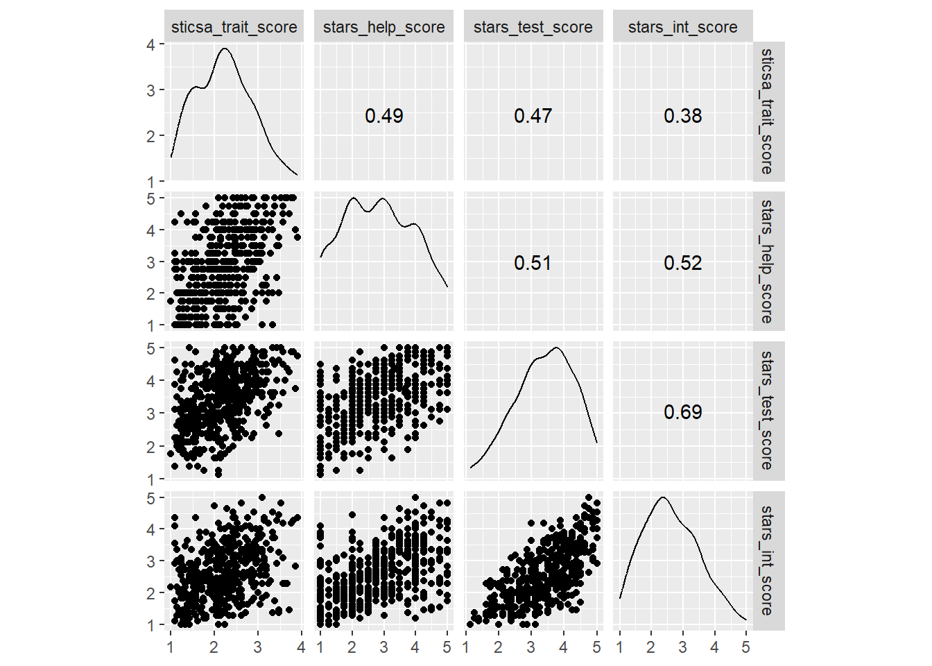
So, this single function gets us a pretty complex plot: a matrix containing all of our variables along the top and side, with density plots on the diagonal, scatterplots on one pairwise intersection, and correlation coefficients on the other.
This is the only {GGally} function we teach in UG at Sussex, but to go a bit further, there’s another example that might be useful in the future.
Exercise
CHALLENGE: Use GGally::ggpairs() on the same numeric variables, but split up all the plots by gender as well.
Hint: There’s an example of this code in the introduction documentation for the lovely palmerpenguins::penguins dataset!
Solution
The “Exploring Correlations” section of the palmerpenguins document gives an example of this code.
To adapt it, first, remember to select both the grouping variable sticsa_trait_cat AND the numeric outcome variables.
Second, use the aes() function in ggpairs() to assign different colours to the different categories in sticsa_trait_cat. We’ll look at aes() a lot more next week when we get to {ggplot2}.
anx_data |>
  dplyr::select(sticsa_trait_cat, contains("score")) |>
  GGally::ggpairs(aes(color = sticsa_trait_cat))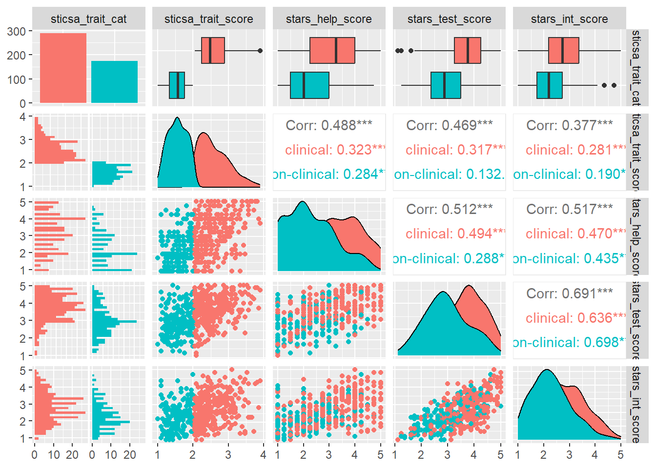
The example of this in the {palmerpenguins} intro document also changes the default colours, which is something we’ll look at when we take a tour through {ggplot2} ourselves.
Testing Correlation
Single Pairwise
If we wanted to perform and report a detailed correlation analysis on a single pair of variables, the easiest function to use is cor.test(). Like t.test() (which we encountered in Tutorial 01/02), this is a {stats} package that works in a very similar way. This is what we teach UGs in first year.
Multiple Pairwise Adjusted
In second year, UGs are also introduced to the (more {tidyverse}-friendly) function correlation::correlation().
Why would you use this one vs cor.test()? On the good side, this function scales up to pairwise tests between as many variables as you give it. This means if you want, for instance, multiple pairwise correlations within a dataset, this is the way to go, since it will apply a familywise error rate correction by default (Holm, to be precise).
On the other hand, it’s a right pain to type and doesn’t play ball with {papaja}. The family of packages that {correlation} belongs to, collectively called {easystats}, has its own reporting package, appropriately called {report} - so pick your poison I guess 🤷6
Unbelievably, we’re actually at the end of this monstrosity. How are you doing? Having fun yet? I hope so (I am!).
We’re now halfway through the Essentials section. In the second half, we’ll be expanding outward from data manipulation to learn {ggplot2} properly, and to speedrun some key analyses for undergraduate dissertations.
See you soon!
Footnotes
Here, “silently” means that R overwrites the existing variable without flagging that it is doing this or asking you if you are sure, so it’s important to be aware of this behaviour (and to know what variables already exist in your dataset).↩︎
Note that averaging Likert data is controversial (h/t Dr Vlad Costin!), but widespread in the literature. We’re going to press boldly onward anyway to not get too deep in the statistical weeds, but if you’re using Likert scales in your own research, it’s something you might want to consider.↩︎
The horror!↩︎
{purrr}, cats, scratch, get it?? I’m hilarious.↩︎
I know this because I teach first year undergraduate statistics and therefore have to, not because it’s, like, particularly obvious on the face of it.↩︎
Look, I like my basic {stats} functions. They all look the same and work the same way, don’t require extra installations or loading, and can be reported nicely with {papaja} or custom functions. I love an
htestobject, me! BUT, you gotta find the functions that do what you need them to do. You won’t always use one or the other - just use the one that makes sense to you and works for the task at hand.↩︎