library(tidyverse)
library(haven)
library(labelled)
library(sjPlot)10: Qualtrics and Labelled Data
Overview
This tutorial will focus on efficient, transparent, and user-friendly techniques for working with data specifically gathered using the Qualtrics survey platform. We will cover how to import and work with labelled data from Qualtrics and how to easily produce a data dictionary straight from the dataset itself.
Acknowledgements
This tutorial was co-conceived and co-created with two brilliant PhD researchers, Hanna Eldarwish and Josh Francis, who contributed invaluable input throughout the process of developing the tutorial. This included collecting commonly asked questions and issues with Qualtrics data analysis; discussing the topics to cover and how best to cover them; and testing code and solutions. Hanna Eldarwish also provided the basis for the dataset, collected during her undergraduate dissertation at Sussex under the supervision of Dr Vlad Costin.
Setup
Packages
As usual, we will be using {tidyverse}. When {tidyverse} is installed, it also installs the {haven} package, which we will use for data importing. However, {haven} isn’t loaded as part of the core {tidyverse} group of packages, so let’s load it separately. Finally, we will also need the {labelled} package to work with labelled data.
Data
Today’s dataset focuses on various aspects of meaning in life (MiL), and has been randomly generated based on a real dataset kindly contributed by Hanna Eldarwish and Vlad Costin. All variables have been randomly generated, but they are based on the patterns in the original dataset. The original, bigger dataset will be made available alongside article publication in the future, so keep an eye out for it!
New File Type
You might notice that instead of the familiar readr::read_csv(), today we have haven::read_sav(). That’s because the file I’ve prepared is a SAV file, associated with the SPSS statistical analysis programme. The next section explains why we are using this data type, but otherwise, there’s nothing new about these commands.
Codebook
This codebook is intentionally sparse, because we’ll be generating our own from the dataset in just a moment. This table covers only the questionnaire measures to help you understand the variables.
| Variable Prefix | Scale | Subscale |
|---|---|---|
| global_meaning | Meaning in Life | Global Meaning |
| mattering | Meaning in Life | Mattering |
| coherence | Meaning in Life | Coherence |
| purpose | Meaning in Life | Purpose |
| sym_immortality | Symbolic Immortality | Single scale |
| belonging | Belonging | Single scale |
Qualtrics Data
Qualtrics is a survey-building tool very commonly used for questionnaire-type studies, as well as some experimental work. The University of Sussex has an institutional licence for Qualtrics, so all staff and students can log in with their Sussex details and easily construct and collaborate on surveys.
For help using Qualtrics itself, the Qualtrics support pages are generally excellent. This tutorial will only briefly touch on the options within Qualtrics itself.
Once the study is complete and responses have been collected, you will need to export your data from Qualtrics so that you can analyse it. Qualtrics offers a variety of export data types, including our familiar CSV type. However, we’re going to instead explore a new option: SAV data.
SAV Data
The .sav file type is associated with SPSS, a widely used statistical analysis programme. So, why are we using SPSS files when working in R?
Importing via .sav has two key advantages. First, it results in a much cleaner import format. If you try importing the same data via .csv file, you’ll find that you need to do some very fiddly and pointless cleanup first. For instance, the .csv version of the same dataset will introduce some empty rows that have to be deleted with dplyr::slice() or similar. The .sav version of the dataset doesn’t have any comparable formatting issues.
Most importantly, however, importing .sav file types into R with particular packages like {haven} gets us a dataset with a special type of data: namely, labelled data. The labels allow us to preserve important information about the questions asked and response options in Qualtrics, and to (mostly) painlessly create codebooks for datasets. We will explore these features in depth in this tutorial.
Exporting from Qualtrics
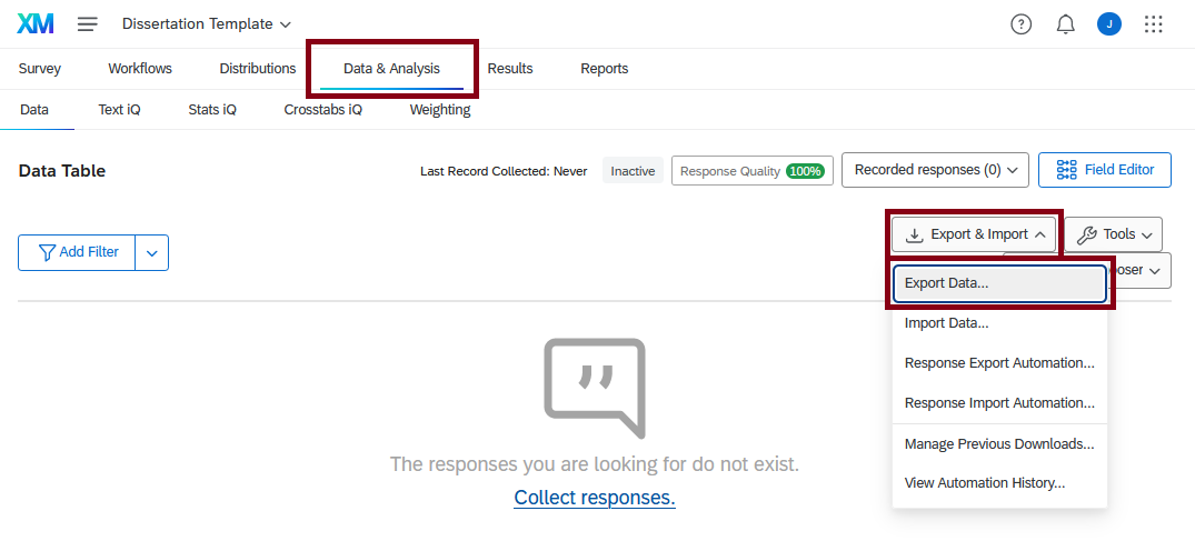
If you’d like to work with your own study data, you will need to export your data in SAV format from Qualtrics first. To do this, open your Qualtrics survey and select the “Data & Analysis” tab along the top, just under the name of your survey.
In the Data Table view, look to the right-hand side of the screen. Click on the drop-down menu labelled “Export & Import”, then select the first option, “Export Data…”
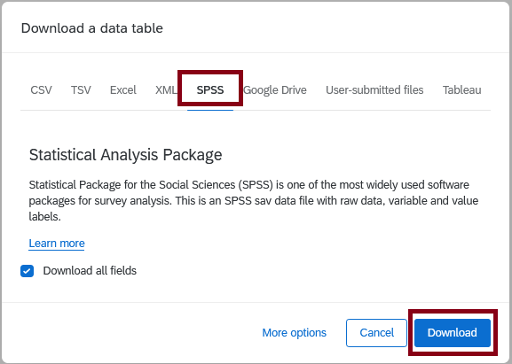
In the “Download a data table” menu, choose “SPSS” from the choices along the top. Make sure “Download all fields” is ticked, then click “Download”.
The dataset will download automatically to your computer’s Downloads folder. From there, you should rename it to something sensible and move it into a data folder within your project folder. From there, you can read it in using the here::here() |> haven::read_sav() combo that we saw in the Data section previously.
Sensible Naming Conventions and Folder Structure
I know it may not seem like something anyone should care about, but sensible file and folder names will make your life so much easier for working in R (and generally).
For folder structure, make sure you do the following:
- Always always ALWAYS use an R Project for working in R.
- Have a consistent set of folders for each project: for example,
images,data, anddocs. - Use sub-folders where necessary, but consider using sensible naming conventions instead.
For naming conventions, your file name should make it obvious what information it contains and when it was created, especially for datasets like this. Personally, I would prefer longer and more explicit file names over brevity; this is because I prefer to navigate files using R, and that’s much easier using explicit file names than it is with file metadata.
So, for a download like this, I’d probably name it something like qtrics_diss_2023_11_08.sav. The qtrics tells me it’s a Qualtrics export, the diss tells me it’s a dissertation project, and the last bit is the full date in easily machine-readable format. Imagine if I continue to recruit participants and download a new dataset later, say a month from now, and name it qtrics_diss_2023_12_08.sav. I could easily distinguish which dataset was which by the date, but also see that they are different versions of the same thing by their shared prefix.
This is a much more reliable system than calling them, say, Qualtrics output.sav and Dissertation FINAL REAL.sav. This kind of naming “convention” contains no information about which is which or when they were exported, or even that they’re two versions of the same study dataset! It might seem like a small detail at the time, but Future You trying to figure out which dataset to use weeks or months later will feel the difference.
The Plan
Our workflow for this dataset will be slightly different than previously. We’ll start by doing some basic cleanup of the dataset, and produce a codebook, or “data dictionary”, drawing on the label metadata in the SAV file. For the purpose of practice, we’ll also have a look at how to work with those labels, and manage different types of missing values.
As useful as labels are, they will get in the way when we want to work with our dataset further. So, we’ll convert the variables in the dataset into either factors, for categorical data, or numeric, for continuous data 1. From that point forward, we can work with the dataset using the techniques and functions we’ve learned thus far.
Cleanup and Data Dictionary
Tip
Most of the following examples are drawn from the “Introduction to labelled” vignette from the {labelled} package. If you want to do something with labelled data that isn’t covered here, that’s a good place to start!
Let’s start off by having a look at the dataset. As usual, you can call the dataset or use View() on it directly, but we’re going to take advantage of the new data type to get a more helpful summary, that emulates the “Variable View” in SPSS.
What we get is a new summary dataset that contains some useful information about each of the variables in mil_data. Along with the actual variable name in the dataset, which we see under variable, we also get the actual question that participants saw in Qualtrics under label, and the response options - where applicable - in value_labels.
Why a data dictionary? There’s two key reasons to do this. First, as we’ve already seen throughout these tutorials, data dictionaries (or “codebooks”) are very useful for understanding datasets, even your own. In this case, we’ve generally named our variables usefully in Qualtrics before the export, but if you forget to (or don’t typically) do this, this reference helps you navigate unhelpful variable names like “Q42”, “Q16” etc. The second reason is for other people: if you want to share your data publicly, including a dictionary/codebook is not only a kindness to other users but also helps prevent misuse or misunderstandings.
Before we look at these labels in more depth, we’re first going to address two minor issues that commonly come up with Qualtrics data to make sure our dataset is ready to use.
Renaming Variables
If you inspected the dataset closely, you might have noticed that one of the items has a strange name: coherence_42, right between coherence_1 and coherence_3.
This wasn’t intentional - in the process of creating the questionnaire in Qualtrics, this variable came out with a weird name. It happens more easily than you think! The best-case option would be to update the Qualtrics questionnaire itself before exporting the data, but you may not be able (or want) to do this, so instead, let’s have a quick look at how to rename variables.
As (almost) always, there’s a friendly {dplyr} function to help us with our data wrangling. This time it’s sensibly-named dplyr::rename(), which renames variables using new_name = old_name arguments.
Tip
Do you have lots of variables to rename? Do you like writing functions, or using regular expressions? Check out rename()’s flashier cousin rename_with(), which uses a function to rename variables.
Separating Columns
The second thing I’d like to do doesn’t concern the main dataset, but rather the data dictionary we’ve generated. For the single-item questions, the label column is reasonably helpful. However, the items with a shared prefix all come from the same matrix scale in Qualtrics, and their labels have two parts: the “question text” that usually contains directions about how to respond, and the actual item text for each individual item.
As an example, the label for belonging_1 reads:
Please rate the extent to which these statements apply to you. - When I am with other people, I feel included
Which corresponds to this in Qualtrics:
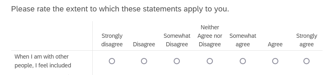
To make the labels more readable, let’s split up the question text, which is repeated for all items on the same subscale and not very useful, and the item text, which contains the specific text of each item. The good news is that the two pieces are defined, or delimited, by the ” - ” symbol that Qualtrics automatically adds to link them.
Since we want to separate the labels column into two - making the dataset wider - using a delimiter, the separate_wider_delim() function from the {tidyr} package should do the trick!
1mil_data |>
2  labelled::generate_dictionary() |>
3  tidyr::separate_wider_delim(
4    cols = label,
5    delim = " - ",
6    names = c("label", "item_label"),
7    too_few = "align_start"
)- 1
- Take the data, and then
- 2
- Generate the data dictionary, and then
- 3
- Separate wider by delimiter as follows:
- 4
-
Separate the
labelcolumn - 5
- At the ” - ” delimiter
- 6
- Into two new columns called “label” and “item_label” respectively
- 7
- If there are too few pieces (that is, for the rows where there is no delimiter), fill in values from the start.
The result isn’t perfect, but it’ll do for our purposes - namely, to have a quick reference for the variables in our dataset.
Viewer Data Dictionary
I personally like labelled::generate_dictionary() because (you will be unsurprised to learn) I like to mess about with regex to make it read just as I like. However, if you primarily need a quick reference as you’re working with your dataset, the delightful sjPlot::view_df() function makes this particularly easy.
Labelled Data
As we’ve just seen in the data dictionary, the SAV data we’re using has a special property: labels. Labelled data has a number of features, all of which we will explore in depth shortly:
Variable labels. The label associated with a whole variable will contain the text of the item that the participants responded to. This is analogous to the “Label” column of the Variable View in SPSS.
Value labels. The label associated with individual values within a variable will contain the text associated with individual choices, for instance the points on a Likert scale or the options on a multiple-choice question. This is analogous to the “Values” column of the Variable View in SPSS.
Missing values. Within value labels, you can designate particular values as indicative of missing responses, refusal to respond, etc. This is analogous to the “Missing” column of the Variable View in SPSS.
We’re first going to look at how you can work with each of these elements. The reason to do this is that once our dataset has been thoroughly checked, we’re going to generate a final data dictionary, then convert any categorical variables into factors, the levels of which will correspond to the labels for that variable. We’ll also convert any numeric variables into numeric data type, which will discard the labels; that will make it possible to do analyses with them, but that’s why we have to create the data dictionary first.
Important
These features will work optimally only if you have set up your Qualtrics questionnaire appropriately. Make sure to refer to the Setting Up Qualtrics section of the next tutorial to get the most out of your labelled data and save yourself data cleaning and wrangling headaches later.
Variable Labels
Variable labels contain information about the whole variable, and for Qualtrics data, will by default contain either an automatically generated Qualtrics value (like “Start Date”), or the question text that that variable contains the responses to.
Getting Labels
To begin, let’s just get out a single variable label to work with using labelled::var_label().
To specify the variable we want, we will need to subset it from the dataset, using either $ or dplyr::pull() as previously.
labelled::var_label(mil_data$gender)[1] "What is your gender identity?\n\nThis question is optional. - Selected Choice"Creating/Updating Labels
If you’d like to edit labels, you can do it “manually” - that is, just writing a whole new label from scratch.
The structure of this code might look a little unfamiliar in terms of the code structure. For the most part, we’ve seen code that contains longer and more complex instructions on the right-hand side of the <-, and a single object being created or updated on the left-hand side. In the structure below, the left-hand side contains longer and more complex code that identifies the value(s) to be updated or created, and the right-hand side contains the value(s) to create or update. It’s the same logic, just with a different structure.
labelled::var_label(mil_data$StartDate) <- "Date and time questionnaire was started"

labelled::var_label(mil_data$StartDate)
[1] "Date and time questionnaire was started"If you’re up for it, though, I’d recommend using it as an opportunity to start working with regular expressions. For example, if we want to keep only the first bit of the label for gender, then we can keep everything only up to an including the question mark, and and re-assign that to the variable label. This style is a bit more dynamic and resilient to changes or updates.
labelled::var_label(mil_data$gender) <- labelled::var_label(mil_data$gender) |>
  gsub("(.*\\?).*", "\\1", x = _)

labelled::var_label(mil_data$gender)
[1] "What is your gender identity?"Searching Labels
A very nifty feature of variable labels and {labelled} is the ability to search through them with labelled::look_for(). With the whole dataset, look_for() returns essentially the same info as generate_dictionary(), but given a second argument containing a search term, you get back only the variables whose label contains that term.
Value Labels
Value labels contain individual labels associated with unique values within a variable. It’s not necessary to have a label for every value, and indeed sometimes it’s advantageous not to.
Getting Labels
There are two functions to assist with this. labelled::val_labels() (with an “s”) returns all of the labels, while labelled::val_label() (without an “s”) will return the label for a single specified value.
labelled::val_labels(mil_data$english_fluency_1) Very well Well Not well Not at all
1 2 3 4 labelled::val_label(mil_data$english_fluency_1, 3)[1] "Not well"Creating/Updating Labels
These two functions can also be used to update an entire variable or a single value respectively. The structure of this code is the same as we saw with variable labels previously.
Missing Values
Labelled data allows an extra functionality from SPSS, namely to create user-defined “missing” values. These missing values aren’t actually missing, in the sense that the participant didn’t respond at all. Rather, they might be missing in the sense that a participant selected an option like “don’t know”, “doesn’t apply”, “prefer not to say”, etc.
Let’s look at an example. As we’ve just seen, we can get out all the value labels in variable with labelled::val_labels():
labelled::val_labels(mil_data$english_fluency_1) Very well Well Not well Not at all
1 2 3 4 This variable asked participants to indicate their level of English fluency. Even for participants who have in fact responded to this question, we may want to code “Not well” and “Not as all” as “missing” so that they can be excluded easily. To do this, we can use the function labelled::na_values() to indicate which values should be considered as missing.
labelled::na_values(mil_data$english_fluency_1) <- 3:4

mil_data$english_fluency_1
<labelled_spss<double>[164]>: Please select which box best describes your English fluency. - How well can you speak English?
[1] 2 2 2 1 1 1 2 1 2 1 1 1 1 1 1 1 1 1 1 1 1 1 1 1 1 1 1 1 1 1 1 1 1 2 1 1 1
[38] 1 1 1 1 1 1 1 1 1 1 1 1 1 1 1 2 1 1 1 1 1 1 1 1 2 1 1 1 2 1 1 1 1 2 1 1 1
[75] 1 1 1 2 1 1 1 1 1 1 1 1 1 1 1 1 1 1 1 1 1 1 1 1 2 1 1 1 2 1 1 1 1 1 1 2 2
[112] 1 1 1 1 1 1 1 1 1 1 1 1 1 1 1 1 1 2 2 1 1 1 1 1 1 1 1 1 1 1 1 1 1 1 1 1 1
[149] 1 1 1 1 1 1 1 1 1 2 1 1 1 1 3 2
Missing values: 3, 4
Labels:
value label
1 Very well
2 Well
3 Not well
4 Not at allFor the moment, these values are not actually NA in the data - they’re listed under “Missing Values” in the variable attributes. In other words, the actual responses are still retained. However, if we ask R which of the values in this variable are missing…
is.na(mil_data$english_fluency_1) [1] FALSE FALSE FALSE FALSE FALSE FALSE FALSE FALSE FALSE FALSE FALSE FALSE
[13] FALSE FALSE FALSE FALSE FALSE FALSE FALSE FALSE FALSE FALSE FALSE FALSE
[25] FALSE FALSE FALSE FALSE FALSE FALSE FALSE FALSE FALSE FALSE FALSE FALSE
[37] FALSE FALSE FALSE FALSE FALSE FALSE FALSE FALSE FALSE FALSE FALSE FALSE
[49] FALSE FALSE FALSE FALSE FALSE FALSE FALSE FALSE FALSE FALSE FALSE FALSE
[61] FALSE FALSE FALSE FALSE FALSE FALSE FALSE FALSE FALSE FALSE FALSE FALSE
[73] FALSE FALSE FALSE FALSE FALSE FALSE FALSE FALSE FALSE FALSE FALSE FALSE
[85] FALSE FALSE FALSE FALSE FALSE FALSE FALSE FALSE FALSE FALSE FALSE FALSE
[97] FALSE FALSE FALSE FALSE FALSE FALSE FALSE FALSE FALSE FALSE FALSE FALSE
[109] FALSE FALSE FALSE FALSE FALSE FALSE FALSE FALSE FALSE FALSE FALSE FALSE
[121] FALSE FALSE FALSE FALSE FALSE FALSE FALSE FALSE FALSE FALSE FALSE FALSE
[133] FALSE FALSE FALSE FALSE FALSE FALSE FALSE FALSE FALSE FALSE FALSE FALSE
[145] FALSE FALSE FALSE FALSE FALSE FALSE FALSE FALSE FALSE FALSE FALSE FALSE
[157] FALSE FALSE FALSE FALSE FALSE FALSE TRUE FALSE…we can see one TRUE corresponding to the 3 above.
If we wanted to actually remove those values entirely and turn them into NAs for real, we could use labelled::user_na_to_na() for that purpose. Now, the variable has only two remaining values, and any 3s and 4s have been replaced.
labelled::user_na_to_na(mil_data$english_fluency_1)<labelled<double>[164]>: Please select which box best describes your English fluency. - How well can you speak English?
[1] 2 2 2 1 1 1 2 1 2 1 1 1 1 1 1 1 1 1 1 1 1 1 1 1 1
[26] 1 1 1 1 1 1 1 1 2 1 1 1 1 1 1 1 1 1 1 1 1 1 1 1 1
[51] 1 1 2 1 1 1 1 1 1 1 1 2 1 1 1 2 1 1 1 1 2 1 1 1 1
[76] 1 1 2 1 1 1 1 1 1 1 1 1 1 1 1 1 1 1 1 1 1 1 1 2 1
[101] 1 1 2 1 1 1 1 1 1 2 2 1 1 1 1 1 1 1 1 1 1 1 1 1 1
[126] 1 1 1 2 2 1 1 1 1 1 1 1 1 1 1 1 1 1 1 1 1 1 1 1 1
[151] 1 1 1 1 1 1 1 2 1 1 1 1 NA 2
Labels:
value label
1 Very well
2 Well
Tip
See the {labelled} vignette for more help on working with user-defined NAs, including how to deal with them when converting to other types.
Converting Variables
The labels have served their purpose helping us navigate and clean up the dataset, and produce a lovely data dictionary for sharing. However, if we want to use the data, we’ll need to convert to other data types that we can use for statistical analysis.
This will fall into two main categories. Any variables containing numbers that we want to do maths with, we’ll convert to numeric type, which we’ve encountered a few times before, which will strip the labels. However, any variables that contain categorical data, we’ll instead convert to factors, which we haven’t encountered in this series yet - so we’ll start there. Remember that variables that will be converted to factor should have labels for all of their levels, whereas variables that will be converted to numeric can have fewer labels, because we will stop using them after the numeric conversion.
Factor
Factor variables are R’s way of representing categorical data, which have a fixed and known set of possible values. Thus far we’ve mostly been using character data for this purpose, but that’s a bit of a cheat - R’s been helping us by treating the same values as the same category, but factors create this structure explicitly.
As may be familiar from SPSS, factors actually contain two pieces of information for each observation: levels and labels. Levels are the (existing or possible) values that the variable contains, whereas labels are very similar to the labels we’ve just been exploring.
As an example, take an example factor vector:
factor(c(1, 2, 1, 1, 2),
       labels = c("Male", "Female"))
[1] Male Female Male Male Female
Levels: Male FemaleThe underlying values in the factor are numbers, here 1 and 2. The labels are applied to the values in ascending order of those values, so 1 becomes “Male”, “2” becomes “Female”, etc. Here, we haven’t need to specify the levels; if you don’t elaborate otherwise, R will assume that they are the same as the unique values.
You can also supply additional possible values, even if they haven’t been observed, using the levels argument:
factor(c(1, 2, 1, 1, 1),
       levels = c(1, 2, 3),
       labels = c("Male", "Female", "Non-binary"))
[1] Male Female Male Male Male
Levels: Male Female Non-binary
Tip
Factors are so common and useful in R that they have a whole {tidyverse} package to themselves! You already installed {forcats} with {tidyverse}, but you can check out the help documentation if you’d like to learn more about working with factors.
The useful thing about labelled data that it’s very easy to convert into factors, which is what R expects for many different types of analysis and plotting functions. Handy!
For an individual variable, we can use labelled::to_factor() to convert to factor.
If you wanted a specific order of the levels, for plotting or similar, there’s also a sort_levels = argument described in the help documentation.
Numeric
For continuous variables, we don’t need anything fancy to turn them into numeric data, because they technically already are. Instead, we just need to get rid of the labels using unclass().
The nice thing about this method is that we can now do maths with the unclassed numeric functions as normal, but the labels are still there if we want to get back - just convert with labelled::labelled().
Conditional Conversion
There are two main ways we could more efficiently convert variables than one by one. The first is offered by the {labelled} package - here I’ve just copied from the vignette describing the setup.
Note
In most of cases, if data documentation was properly done, categorical variables corresponds to vectors where all observed values have a value label while vectors where only few values have a value label should be considered as continuous.
In that situation, you could apply the unlabelled() method to an overall data frame. By default, unlabelled() works as follows:
- if a column doesn’t inherit the
haven_labelledclass, it will be not affected; - if all observed values have a corresponding value label, the column will be converted into a factor (using
to_factor()); - otherwise, the column will be unclassed (and converted back to a numeric or character vector by applying
base::unclass()).
If we wanted to do this, we’d have a bit more work to do. That’s because at the moment, our data doesn’t line up with this template. Having a look at our data dictionary again, we can see that our subscale variables have all of their levels labelled, so they won’t be converted as we’d like. Rather than do this now, I’d probably recommend setting up your Qualtrics like this to begin with.
Instead, we can take the second route and use what we’ve seen in previous Challenge tasks to convert variables conditionally.
Very well done today. You should now have a data dictionary to refer to, and a complete dataset to work with using the techniques we’ve already covered to clean up responses, create subscales, and so on. Next time we’ll work on solving common issues and avoiding those issues in the first place by setting things up right to begin with.
Footnotes
For the purposes of simplicity, we’re going to keep pretending that Likert and similar rating scales are “continuous”.↩︎