## Keysmash!
aslavb;lj aew aljvb
Error: <text>:2:11: unexpected symbol
1: ## Keysmash!
2: aslavb;lj aew
^
Welcome to the first PsychRlogy tutorial! Let’s jump right in and get started.
This tutorial is designed to accompany a “Workbook” document, which is already available for you on the Posit Cloud workspace for this course. To access it, navigate to Posit Cloud and open the course workspace. If you haven’t joined the workspace yet, use the join link on the Posit Cloud page on Canvas.
In the workspace, you will see a list of projects available. These will have an “ASSIGNMENT” banner next to them. When you click on these projects, a new copy of the project will be generated for you to work in.
You are now looking at the RStudio IDE itself. It is possible to use R directly with minimal interface, but using an integrated development environment like RStudio comes with a lot of additional convenience to make working with R smoother, easier, and more efficient.
It’s beyond the scope of this tutorial to cover all of the options and tools available in RStudio. Here we’ll focus only on the minimum to get started and build outward from there.
For a more complete tour, try this playlist of Andy Field’s RStudio tutorials.
Before anything else, open up the workbook for this tutorial. If you’re a little shaky on where this is, skip down to the screenshot below!
You should now be looking at a dashboard-like interface with four main windows, each with a bunch of tabs across the top, like pictured below. We’ll refer to each window by these names, which come from the most important or commonly used tab in each window.
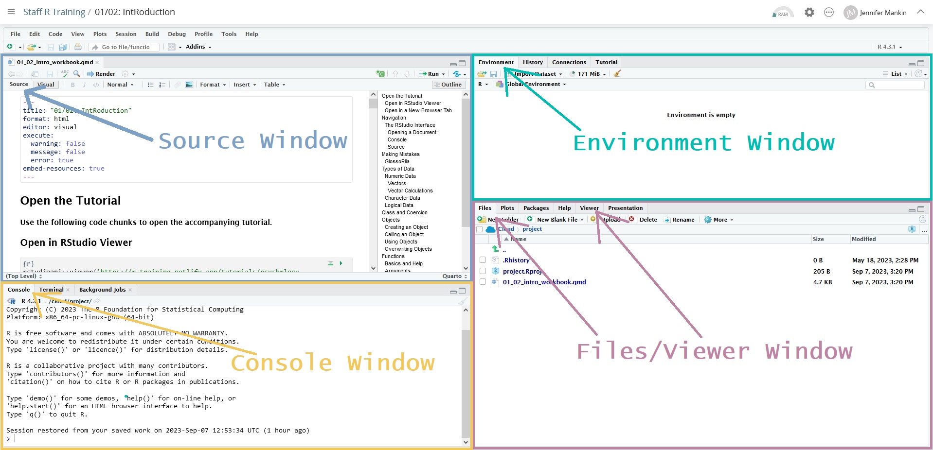
We will eventually work with all four of these windows, but if you’ve opened the workbook, you can ignore the Environment and Files windows for now. We’ll be focusing only on the other two: Source and Console.
The Source window is where any documents you want to create or work on will open up. What you have open now is a Quarto document, a type of document that integrates regular text and code. A Quarto document has three main elements: the YAML header, body text, and code chunks.
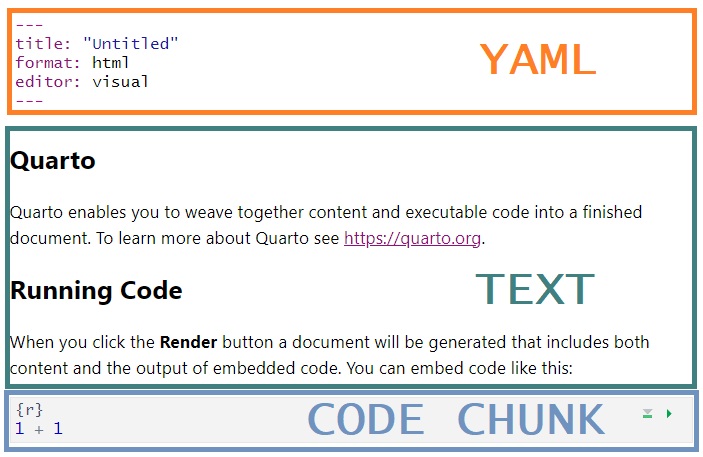
Ignore the YAML header for now; we’ll come back to Quarto documents, including the YAML, in depth in Tutorial 04.
You can use the body text portion of a Quarto document more or less like you would a document in Word (or your word processor of choice). In the body of the document, you can write and format any text you want - notes, questions, thoughts, ideas, comments, etc. This workbook already contains all the headings from this tutorial to help you get organised, but please do delete or edit as you see fit.
The last element is the code chunk, which is where all R code should be written. Code chunks have a contrasting background colour, an {r} in the upper left corner, and two green buttons in the upper right. The one that looks like a green “play” button will run all the code in that chunk. Code chunks will NOT handle any non-code text, unless it’s a comment (i.e. preceded by one or more #s.)
The Console is deceptively simple: just some stuff about the R version and acknowledgements, and the > symbol with a flashing cursor after it, waiting for you to type something. However, the Console is the heart of R, where anything you want to do actually happens. Every command that you type, anything you want R to do, goes through here.
So, already we have two places we could write R code: in a code chunk or in the Console. How do we know where to start?
For the purposes of learning, by default, it’s best that you write all code into the workbook code chunks, so you have a detailed record of everything you’ve tried - even if it doesn’t work!
Outside of these sessions, whether to write a bit of R code in a code chunk in Quarto, or in the Console, largely depends on a single question: do you want to use this same line of code again in the future?
If yes, write the code in a code chunk. By adding the code to a document like Quarto, we are creating a record of all the steps we’ve taken in whatever task we are working on. Assuming we want to be able to use and refer to that code again in the future, it should go into a document.
If no, write the code in the Console. Code written directly in the Console isn’t saved or documented anywhere1. Some common uses of the Console are:
So, I often use the Console to test my code, building it up bit by bit, until it does what I want it to do. Then, when I’ve puzzled out the solution, I add it into a code chunk.
Imagine that working in R is like cooking, and writing a sequence of commands to, for example, clean a new dataset is like developing a new recipe.
If you’re developing a recipe, you likely wouldn’t just sit down and write down the final version if you’ve never tried the recipe before. Instead, you might experiment a bit with each step to see what works and what doesn’t.
Along the way, you may write notes to yourself: “Maybe try cumin?”, “Buy more kefir”, “This time was 2 tsp salt, too salty!” Those notes are a part of the development process, relevant to what you’re doing now and helpful to try out or note down ideas, but they wouldn’t go in your final recipe. Those behind-the-scenes and under-development bits are the code you’d write in the Console.
When you find a technique or temperature or seasoning that works, you might add it as a step in your recipe. That final recipe, the steps that actually work the way you want, are the code in your code chunks.
If that seems like a lot to remember, don’t worry - we’ll practice both and let you know clearly if it should be one or the other.
Right, enough orientation - let’s get cracking!
Before we go any further, an affirmation: you will, inevitably, make typos and errors using R. You will write commands that make sense to you that R doesn’t understand; and you will write commands that don’t make sense to you, that R does understand. Errors are an essential and unavoidable part of learning R, so let’s start there.
Well, that went about as well as expected.
If you haven’t tried this yet, and your pristine document is just ominously staring at you, I’m serious - punch your keyboard if you have to, or let your cat walk on it, or play it as if it were a piano, and press Enter. There’s two important things to learn from this:
To ask R to do something, you must write commands out somewhere (in a code chunk, in the Console) and then run them.
Eventually, inevitably, something that you type WILL produce an error.
From our keysmashing above, you will have seen that aslavb;lj aew aljvb, Am I a coward? Who calls me villain?, and ¯\_(ツ)_/¯ are not valid commands in R. Although each of these has a communicative function for humans, R can’t understand them. In order to get the answer that we want, we have to ask R to do something in a way it can understand, by writing commands it can parse using the R language.
Just like learning any other language, learning to communicate with R takes time and practice, and it can be very frustrating when you and R can’t seem to understand each other. However, one advantage of learning to talk to R vs learning to speak a human language is that R always works the same way. Even if the response it gives doesn’t make sense to you, there’s always a logical reason for what it does.
Very often, R communicates with you via errors. Unlike many other computer programmes you might be familiar with, an “error” in R doesn’t (usually!) mean a catastrophic failure and/or potential loss of hours of work2. Rather, whatever you’ve asked R to do, it’s essentially replied, “Sorry, I can’t do that.” Two of the most important skills you can develop early on with R is to treat errors as feedback, and to learn to read and recognise errors.
Treat errors as feedback: Errors aren’t (just) an annoyance, although running into lots of errors, usually just when you don’t want them the most!, can be incredibly frustrating. However, errors are just R’s way of telling you that it can’t do what you’ve asked it to do. If you’re trying to work out how to get R to do something, then the “no” of an error rules out whatever you’ve just tried. Rather than setting out to avoid errors, and thinking of an error as a “failure” to “do it right”, it’s much better to expect errors, and make use of them as part of the code-writing process.
Learn to read and recognise errors: Errors often contain useful information about what’s gone wrong and how to fix it. At minimum, errors usually contain the following information:
Errors vary wildly in understandability and helpfulness, from highly technical jargon to friendly and conversational with suggestions for fixing common problems. Even the obtuse ones, though, will become familiar with time.
Let’s take a look at how we might interpret the error we produced above.
aslavb;lj aew aljvbError: <text>:1:11: unexpected symbol
1: aslavb;lj aew
^Here R doesn’t need to tell us where the error is, because there’s only one thing it’s trying to run. We do have the text of the error, though: object 'aslavb' not found. We’ll come to objects later on in this tutorial, but in short R is looking for some information labeled aslavb and can’t find it (because it’s just a keysmash!). This is an example of an error that comes up all the time - often when you’ve made a typo, or forgotten to create or store information in an object properly. For me at this point, as someone who forgets or mistypes things on the reg, this error is a familiar friend!
One key concept for using R is the different ways it categorises data. “Data” here means any piece of information you put into R - a word, a number, the result of a command or calculation, a dataset, etc. Depending on the type of data you have, R will treat it differently, and some operations only work on certain types of data. So, let’s have a look at how R encodes and deals with different types of data. Here we’ll cover three of the most common and important: numeric, character, and logical. As we do so, we’ll practice some core skills in R.
The first, and perhaps most obvious, type of data in R is numbers. We’ll start by doing some calculations with common mathematical operators.
Remember that you can run all the code in a code chunk by pressing Ctrl/Cmd + Shift + Enter on your keyboard, or by clicking the green “play” arrow in the top right corner of the code chunk.
You can also run only a particular line of code, or something that you’ve highlighted, by pressing Ctrl/Cmd + Enter.
This might be what you’d expect. We’ve essentially asked R, “Give me 3958” (or whatever number you put in) and R obliges. The only thing that might be a surprise is the [1] marker, called an index. Basically, R has replied, “The first thing ([1]) that you asked me for is 3958.” We’ll come back to indices in a moment.
So, commas within numbers throw an error. This is because commas have an important role to play in the syntax of R, so long numbers must be inputted into R without any punctuation. However, full stops to mark decimal places are just fine.
Try for a moment switching to Source mode by clicking the Source button in the upper left hand of your Quarto document. You can see that RStudio helpfully marks out the part of the code that isn’t parsable (not in “grammatical” R) with a red ❌ next to the line number, and squiggly red underlining, likely familiar from word processing programmes, under the part of the code that’s causing the issue. It won’t do this for every error, but it’s very helpful for finding “grammatical” errors like extra or missing brackets or misplaced commas.
Next, let’s try doing some maths.
Important to note here is that we don’t need to type an = to get the answer, just the equation we want to solve and then run the code. Again, we’ve asked R, “Give me 40 + 8” (or whatever numbers you chose) and R replies with the answer.
You will not be surprised to learn that you can use R as a calculator to subtract, divide, and multiply as well.
This exercise also shows us something useful: you can run multiple commands within the same code chunk. While spaces are not meaningful to R (that is, 40 - 8 and 40-8 and 40 -8 are all read the same way), new lines have an important role to play separating out commands. Each command must have its own new line.
Let’s imagine I am running a study, and I want to generate some simple participant ID numbers to keep track of the order that they completed my study. I had 50 participants in total. I could do this by typing every number out one by one, but this is exactly the kind of tedious nonsense that R is great at. Instead, we’ll use the operator :, which means “every whole number between”.
Notice that the indices mentioned earlier have come up again. The first element after the [n] index is the nth element. Let’s have a look at this some more.
You may have tried something like this:
12:30 [1] 12 13 14 15 16 17 18 19 20 21 22 23 24 25 26 27 28 29 3023:55 [1] 23 24 25 26 27 28 29 30 31 32 33 34 35 36 37 38 39 40 41 42 43 44 45 46 47
[26] 48 49 50 51 52 53 54 5536[1] 36As you can see from the indices, this is three separate commands, because the numbered indices start over from [1] each time. However, we want all those numbers in a single command. To do this, we’ll use a function called c().
This is our first contact with functions in R, and we’ll explore how they work more later on. To use this one, type it out, then inside the brackets, put the numbers you want to collect (or concatenate, or combine), with different groups separated by commas.
c(12:30, 23:55, 36) [1] 12 13 14 15 16 17 18 19 20 21 22 23 24 25 26 27 28 29 30 23 24 25 26 27 28
[26] 29 30 31 32 33 34 35 36 37 38 39 40 41 42 43 44 45 46 47 48 49 50 51 52 53
[51] 54 55 36As you can see from the numbered indices this time, when I put the numbers I want inside the function c(), separated by commas, R collects all of the numbers into a single series of elements, called a vector.
Actually, we’ve been looking at vectors this whole time. Any series of pieces of information in R is a vector (but see Tip box on vectors and elements). When we were looking at single numbers (like 3958 above), we were still getting a vector back from R, but it was a vector with only one element, and thus only [1].
If I want the nth element in the vector we’ve just created, (say, the 33rd), I can get it out by indexing with square brackets.
c(12:30, 23:55, 36)[33][1] 36What I’ve essentially asked R is, “Put all of these numbers into a single vector, and then give me the 33rd element in that vector.” As it turns out, the 33rd element in that vector of numbers is 36.
A vector is essentially a series of pieces of data, or elements. It is a key basic piece of how data is stored in R. When R returns a vector as the output from a command, each element is numbered in square brackets. These square brackets can also be used to index the vector to get the nth element.
For atomic vectors created with c() or similar operations, there are some important rules:
For a complete explanation of vectors (and their more versatile siblings, lists) that’s beyond the scope of this tutorial, see:
This could be a very tedious process, but here we have an example of a vectorised operation. By default, the operation “subtract 7” is automatically applied to each individual element of the vector.
We can do a lot more than this with numbers and data in R, but this is an excellent start. Just one note before we move on about the order in which R performs its calculations.
Mathematical expressions are evaluated in a certain order of priority. You can use brackets to tell R which part of a longer calculation to do first, e.g.:
59 * (401 + 821)[1] 72098Without the brackets, the expression is evaluated from left to right, which in this case would give a different answer:
59 * 401 + 821[1] 24480Whenever there’s any chance for ambiguity, always use brackets to make sure the calculation is performed correctly.
Characters are a more general data category that also includes letters and words. In R, strings of letters or words must be enclosed in either ‘single’ or “double” quotes, otherwise R will try to read them as code:
Hello world!Error: <text>:1:7: unexpected symbol
1: Hello world
^"Hello world!"[1] "Hello world!"As you can see here, the first command without quotes throws an error, whereas the second prints out our input just like it did with the single numbers before.
An important thing to note is that R sees everything inside a pair of quotes as a single element, regardless of how long it is. You can see this in the indices we saw before:
"Hi!"[1] "Hi!""It was the best of times, it was the worst of times, it was the age of wisdom, it was the age of foolishness..."[1] "It was the best of times, it was the worst of times, it was the age of wisdom, it was the age of foolishness..."The [1] markers also tell us that each of the two strings above already constitute vectors, each of length 1. Just like we saw with numbers, above, any number of character strings can be combined into a vector. You can also use the numbered markers to extract the nth element in that vector.
The placement of the quotes is very important - they can’t include the commas. As we saw before, R uses commas to separate different elements. So, if you didn’t enclose each word in quotes separately with commas in between, you would have had this odd message:
c("bumblebee, squid, falcon, flea, seagull")[3][1] NANA is a special value in R. It indicates that something is not available, and it usually represents missing data, or that a calculation has gone wrong or can’t be performed properly.
Here, we asked R for the third element in a vector that, as far as R can tell, only contained one. This is because there’s only one pair of quotes, so all five animals and the commas between them are considered to be one element. Since there isn’t a third element, R has informed us so accordingly - the answer to our query is NA, doesn’t exist.
The final type of data that we’ll look at for now is logical data. In addition to performing calculations and printing out words, R can also tell you whether a particular statement is TRUE or FALSE. To do this, we can use logical operators to form an assertion, and then R will tell us the result.
The last few statements above may have caused you some trouble if the notation is unfamiliar.
For “less than or equal to”, R won’t recognise the \(\le\) symbol. Instead, we combine two operators, “less than” < and “equal to” =, in the same order we’d normally read them aloud. The same goes for “greater than or equal to”, >=. (It does have to be this way round; try =< and => to see what happens.)
For “does not equal”, ! is common notation in R for “not”, or the reverse of something. So != can be read as “not-equals”.
For “equals”, if you tried this with a single equals sign, you would have had a strange error:
420 = 42Error in 420 = 42: invalid (do_set) left-hand side to assignmentThe problem is that the single equals sign =, like the comma, has some very specialised syntactic uses, including one equivalent to the assignment operator <-, which we’ll look at shortly. Single equals = also has an important and specific role to play in function arguments. Essentially, = is a special operator that doesn’t assert equivalence. Instead, “exactly equals” in R is “double-equals” (or “exactly and only”), ==.
Here R prints out a value of TRUE or FALSE for each comparison it’s asked to make. So, the first element in the output (TRUE) corresponds to the statement 2 <= 6, the second to 3 <= 6, and so on. This is a vectorised calculation again, as we saw with numeric data before. These vectorised assertions will be absolutely essential to selecting and filtering data that meet particular requirements, or checking our data to find problems.
If you’re a regular SPSS user, you might recognise many of these data types from SPSS. See page 7 of this SPSS user guide for a reminder of these types.
So far, what we’ve called “numeric” in R is also (broadly) “scale/numeric” in SPSS. What we’ve called “character” in R is “string” in SPSS. As far as I know, SPSS doesn’t have an equivalent of “logical”, but would probably be a “nominal/string” type.
We haven’t thus far talked about a few common data types that you might be used to using in SPSS. Ordinal and Nominal data types in SPSS correspond (more or less) to factors in R, which we will come to in a later tutorial. R also has date-time data, which is not covered in this series, but if you need to use it, check out the {lubridate} package.
With these short examples, it may be obvious just by looking that 25 is a number and porcupine is a word. However, this isn’t always so straightforward, and there are some situations - such as data checking/cleaning, or debugging - where we might want to check what type of data a certain thing is. To do this, we’ll need another new function, class(). This function will print out, as a character, the name of the data type of whatever is put into the brackets.
Something interesting has happened here. Recall that atomic vectors created with c() must all have the same data type. Here, we combined two types of data: numeric and character. We didn’t get an error - instead, without warning or telling us, R quietly converted the entire vector to character type. This forcible conversion is called coersion.
Coersion is when a piece of data is forcibly changed from one data type to another. This is sometimes intentional, but it can happen unintentionally (and without any warning or fanfare!), so is a common source of errors.
Coersion follows a hierarchy; data types on the left can be coerced into the types further along to the right.
logical ==> integer ==> double (numeric) ==> character
As we saw previously, you can check the data type of a vector with class(). You can also check if a vector is a particular type (and receive a logical vector in response) with the is.*() family of functions. (The * notation refers to a placeholder for many different options, such as is.numeric, is.character, etc.)
You can similarly (try to) coerce a vector into a particular data type with the as.*() family of functions.
This explains why our vector from the last exercise was a character vector - since the vector contained at least one character element, everything else in the vector was coerced to the same type. This can cause problems when, for example, numeric data is coerced into character data, even though it still looks like numbers.
Even though we can do mathematical operations on numbers, we can’t do them on characters; it should be clear that asking e.g. what is "tomato" - 7 is nonsense. However, this is the case even if all of the data are numerals! For example:
## No problem here; all numbers
c(2:20, 45) - 7
[1] -5 -4 -3 -2 -1 0 1 2 3 4 5 6 7 8 9 10 11 12 13 38## Doesn't work
c(2:20, "45") - 7Error in c(2:20, "45") - 7: non-numeric argument to binary operatorEven though “45” looks like a number, because it’s in quotes, R thinks that it’s a character, and will refuse to do the calculation, in the same way that it would refuse to do it with “tomato”.
Here for the first time we see an example of a warning. Warnings are not errors, even though they get printed out in the same (usually alarming) colour and the same (often unfriendly) curt tone. The key difference is whether the code runs or not. With errors, the code cannot be executed as written, and the error is returned at the point where the execution failed. With warnings, the code CAN be (and has been) executed as written, but R is telling you that it has done something that you might not have expected or wanted along the way.
What we have asked in this command is for three pieces of data to be coerced to numeric type. The first, 20, is already numeric type, so presents no issue. The second, "42", is character type (because of the quotes), but is also parsable as a number so similarly presents no issue. The problem is "36 years old", which cannot be turned into a number3. Instead of throwing an error, though, R instead replaces "36 years old" in the output vector with NA, and prints a warning to let you know it’s done this. If this is what you wanted (and sometimes it might be), you can ignore it, but if you thought that all these ages were already numbers, this warning would be an important flag to investigate your data a bit more thoroughly.
R is a programming language, but (being created by speakers of natural language) it has many features similar or analogous to natural languages. In this section, we’ll cover the basic “grammar” of R, including how R understands what you ask it to do.
In a similar way that the basic unit of many languages is the word4, the basic unit of the R programming language is the object. This section will explore the basics of what an object is and some of their key features in R.
Objects are the basic elements that R is built around - the equivalent of words. An “object” in R is any bit of information that is stored with a particular name. Objects can hold anything, from a single number or word to huge datasets with thousands of data points or complex graphs. These named objects are the main way you, the programmer, can store, retrieve, and interact with information in R.
Although we have done quite a bit in R so far - creating vectors, doing calculations, etc. - you may notice that we haven’t stored this information anywhere. To store the output of code for further use, it needs to be assigned to an object using the assignment operator, <-. Once an object is created, it will appear in the Environment pane.
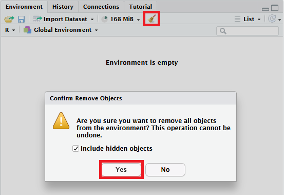
At the moment your Environment should be empty. As a reminder, Environment is by default the first (leftmost) tab in one of your four main windows in RStudio, probably the one on the top right.
If this window is blank except for “Environment is empty”, you’re ready to go. If for some reason it isn’t empty, click the broom icon to clear everything from your Environment before you get started, as indicted in the image below. (There will be a very ominous-sounding “Are you sure?” pop-up, but just click “Yes”.)
First, let’s look at the foundational structure of almost everything you will do in R:
object <- instructionsThis is “pseudo-code”, or a “general format” for a command in R. It isn’t valid R code, but is rather intended as a midpoint between natural language and R to help make it clear how the code works. You can read this code as, “An object is created from (<-) some instructions.”
object: Objects can be named almost anything (although see Naming Objects, below). The object name is a label so you, the analyst, can find, refer to, and use the information you need.<-: The assignment operator <- has single job: to assign output to names, or in other words, to create objects.instructions: Any amount of code that produces some output, which is what object will contain.Generally, you can name objects pretty freely in R. Object names must be a single sequence of symbols, so can’t include spaces or special operators (like =, <-, ,, etc.). The best idea is to come up with naming conventions that work for you, so you can easily remember what objects contain. R will let you know if you try to name an object something that it doesn’t like:
## This doesn't work because it would frankly be bonkers if it did
1285 <- "a"
Error in 1285 <- "a": invalid (do_set) left-hand side to assignment## Can't start with a number...
1stletter <- "a"Error: <text>:2:2: unexpected symbol
1: ## Can't start with a number...
2: 1stletter
^## But numbers inside are okay
letter1 <- "a"
letter1[1] "a"## You can really go wild if you want!
thisis_TheFirstLETTER.of.the.alphabetWOW <- "a"
thisis_TheFirstLETTER.of.the.alphabetWOW[1] "a"In these tutorials, we will typically stick to so-called “snake case” - lowercase names with underscores. This is generally the style of {tidyverse} as well. However, there’s nothing to stop you from using different conventions such as camelCase, PascalCase, whatever.this.is, or mixing them all at random, except maybe for the fact that your future self, and anyone else who might want to read or use your code, will almost certainly despair.
It is actually possible to use unallowable symbols, like spaces and punctuation, in some names, by using backticks. You must use the backticks when you create AND every time you use/call the object. It is generally a very bad idea to do this (just use underscores like a reasonable person), but it occasionally comes in handy for formatting tables or figures when the names don’t need to be machine-readable/good R code/easy to work with anymore.
nope this is bad <- "a"Error: <text>:1:6: unexpected symbol
1: nope this
^`but this one works!` <- "a"
`but this one works!`[1] "a"Assuming your code is valid, you should see a green bar appear along the left-hand side of the code chunk when you run the code, but you might notice that there’s no printout that appears under the code chunk, as there was previously. In fact, if the code ran successfully, it might look like nothing happened at all. To find out what did happen, look your Environment pane. You should now see a new section, “Values”, and underneath the name of your new objects and what they contain. Success!
For any object, from the most simple to the most complex, you can always see what’s in it by calling the object. This simply means that you type the name of the object and run the code. R will print out whatever is stored in the object.
This output looks just like what we saw earlier, when we just asked R to print out a vector of numbers. In essence, the object names are just labels for storing and referring to the information they contain.
These two actions are the essential basis of everything you will do in R. All of your code will, at base, either create an object, or call an object. (Changing an existing object, as we’ll see shortly, is the exact same procedure as creating one from scratch.)
When you create an object using the assignment operator (<-), the object is created but is not printed out. This is because R always does only and exactly what you ask it to do, and using the assignment operator only tells R to assign something to an object, not to print it out6.
When you call an object, the current contents of that object are printed out, but that object is not changed - you only reproduce a copy of its contents for review. To create or change an object, you must use the assignment operator to assign the output to a new (or existing) object name.
Let’s make all of this a bit more concrete by seeing how we can use objects effectively.
Since objects are convenient reference labels for the information they contain, we can work with them as if they were the information they contain. In this case, our objects contain numbers, so we can use them for numerical calculations.
For instance, we might want to know what the mean mark was for this sample of quiz marks. To do this, we could make use of a very handy function, mean(), as follows:
mean(quiz_9am)[1] 51.83333You may have been surprised to see that the class of these objects is numeric, rather than character - even though the name of the object is a character string. To find out the class of the object, R looks at what that object contains, not at the name of the object itself. We already saw that quiz_9am (or whatever your object is called) contains only numbers; so, R tells us that it’s a numeric vector.
One more example to emphasize this point, because it’s often a source of confusion when starting out with R. If we want to ask R the class of the string “quiz_9am”, we would need to put it in quotes, and we’d get a different answer:
class("quiz_9am")[1] "character"The key thing here is that objects have the class of the data they contain, and are not character data; and whenever you want to use an object, you must not use quotation marks. On the other hand, if you want to input character data into R, you must use quotation marks. Otherwise, R will look for an object or function with that name, which will likely produce a “cannot find object” error.
Our last major point to cover with objects - for now - is how to change what an object contains.
The command we’ve just written for the task above demonstrates some extremely important properties of how assignment and functions work in R.
Overwriting objects is accomplished by assigning new output to an existing object name. If you have a look in your Environment, you will see that the previous version of quiz_9am, containing only six values, has been replaced with the new one containing nine values.
Overwriting objects is silent. Unlike, say, a word processor, that will give you a warning if you try to save two documents in the same folder with the same name, R won’t ask you if you’re sure you want to overwrite an existing object with new information - it will just do it. This can be a good thing, because you can easily update the information stored in an object with changes, edits, or new information. However, it also means that you can overwrite or replace data when you don’t want to, if you use the same object name.
This is why it is so important to keep track of all of the commands and changes you make to your data. If you accidentally replace your dataset with, say, a single word, or number with an error in your code, you can easily retrace your steps and avoid redoing work.
Overwriting objects can be done recursively. In the command we saw above, we took the current quiz_9am object, combined it with some new values, and then overwrote the quiz_9am object with the new values. If we were to run this exact same code again, this means that each time we would add three new values to quiz_9am, over and over and over:
quiz_9am <- c(quiz_9am, 89, 100, 79)
quiz_9am
[1] 75 58 62 16 33 67 89 100 79 89 100 79quiz_9am <- c(quiz_9am, 89, 100, 79)
quiz_9am [1] 75 58 62 16 33 67 89 100 79 89 100 79 89 100 79This is one reason why the decision to overwrite an existing object, vs creating a new one, can make a big difference to your code. This behaviour only happens because the input and output objects are the same. If we name the output object something different, we don’t get the same recursion - the new object quiz_9am_full is recreated from the same input in the same way every time, so it always contains the same thing.
## Recreating the original version of quiz_9am so things don't get out of hand!
quiz_9am <- c(75, 58, 62, 16, 33, 67)

quiz_9am_full <- c(quiz_9am, 89, 100, 79)
quiz_9am_full
[1] 75 58 62 16 33 67 89 100 79quiz_9am_full <- c(quiz_9am, 89, 100, 79)
quiz_9am_full[1] 75 58 62 16 33 67 89 100 79There isn’t a right or wrong way to do this - sometimes this recursive property is exactly what you want. (It’s very useful, for example, in loops.) But it is important to be aware of.
Finally, overwriting objects only changes the overwritten objects, and NOT any other objects created from them. To see this in action, recall that earlier we calculated the mean of the two quiz objects and saved it as quiz_diff. If we do the same calculation now with our updated objects, we can see that the difference in the means is no longer the same.
## Value calculated previously
quiz_diff
[1] -5.333333## Value using the updated objects
mean(quiz_9am) - mean(quiz_6pm)[1] 11.44444## Ask R if the two are the same
quiz_diff == (mean(quiz_9am) - mean(quiz_6pm))[1] FALSEThis illustrates the importance of writing and running code sequentially, from beginning to end. If you go back and change values created earlier on in your code, the value you currently have in your Environment may not match the value that your code will produce when run.
If you are interested in understanding this process of assigning and replacing the contents of objects better, the aside below explains it in more depth.
The majority of this aside was originally written by Milan Valášek
Think of objects as boxes. The names of the objects are only labels, and you can store anything you like inside them. However, unlike in the physical world, objects in R cannot truly change. You can put stuff in and take stuff out, and that’s pretty much it. Unlike boxes, though, when you take stuff out of objects, you only take out a copy of its contents. The original contents of the box remain intact. Of course, you can do whatever you want (within limits) to the stuff once you’ve taken it out of the box, but you are only modifying the copy. The key thing to remember is that unless you put that modified stuff into a box, R will forget about it as soon as it’s done with it. In other words, if you want to “save” any changes you make, you must assign them to an object in order to keep them.
Now, as you probably know, you can call your boxes (objects) whatever you want (again, within certain limits). This means that that you can call the new box the same as the old one, as we saw with quiz_9am above. When that happens, R basically takes the label off the old box, pastes it on the new one, and burns the old box. So even though some operations in R may look like they change objects, what’s actually happening is that R copies their content, modifies it, stores the result in a different object, puts the same label on it, and discards the original object. Understanding this mechanism will make things much easier!
Putting the above into practice, this is how you “change” an R object:
# put 1 into an object (box) called a
a <- 1

# copy the content of a, add 1 to it and store it in an object b
b <- a + 1

# copy what's inside b and put it in a new object called a
# discarding ("overwriting") the old object a
a <- b

# now see what's inside of a
# (by copying its content and pasting it in the console)
a
[1] 2Of course, you can just cut out the middleman (creating an object b). So to increment a by another 1, we can do:
a <- a + 1

a
[1] 3
Functions are like verbs in the R language. We’ve already started using a few functions: c(), class(), mean(), and as.numeric(). As we’ve seen, these functions perform some operation using the input inside their brackets, and produce the output of that operation. So, functions are the main way that R does anything.
In this section, we’ll take a systematic look at the process of using a new function - in particular, functions that take multiple inputs, or arguments. As we go, we’ll look at how to “translate” the command you want to give R into a verb (function) it can understand.
Let’s look at an example of how this translation might work. For this example, I’m going to use a number I generated earlier: the mean of the quiz_9am group, 64.3333333, which I’d like to round to two decimal places - a common task for reporting results in APA style.
If we want R to do this for us, we have to write this command in a way that R can understand. First, we need to know what function corresponds to the English verb “round” - that is, what function will do the same action that we want R to perform. We’re lucky in this case: the function in R is also called round().
We know that we’re looking at a function in R because functions often have a name followed by brackets (and nothing else in R does). That is, they have the general form function_name(). Inside the brackets, we can add more information to the function to complete our command, although not all functions require any more information.
What we want to do, “Round the number 64.3333333 to two decimal places”, has two more important pieces of information that we need to tell R: what number we want to round (64.3333333) and how many decimal places we want to round it to (2). So, how do we say this in R? To find out, let’s look at the help documentation.
Help documentation is information, like instruction manuals, built into R about how individual functions work. Function documentation varies wildly in helpfulness and completeness, but it’s a useful place to check first if you want to find out what a function does. You can access the help documentation in a few different ways: by running ?function_name or help(function_name) in the Console, or by clicking on the “Help” tab in the Files section of RStudio and using the Find box to search for the function.
The first section, “Description”, varies quite a bit in intelligibility, depending on how complex the function is. Here, if we ignore the information about the other function included in this document, we can see that we have a useful description of round() that tells us that it rounds numbers (that’s a good sign) to a certain number of decimal places. That’s exactly what we want, so how do we use it?
Let’s scroll down to “Usage”, which gives examples of what the function looks like. You can see that the basic structure of this function is round(x, digits = 0). It seems like we need to add some more information in the brackets of our function - but how do we interpret x and digits = 0?
The information inside a function’s brackets, which give it the information it needs to work, are called arguments. Each argument in a function is separated by a comma, so we can see from round(x, digits = 0) that the round() function can take two arguments. How many arguments a function has depends on the function; some (like Sys.Date()) don’t need any arguments to run. One of the most useful parts of a function’s help documentation is the “Arguments” section, which tells you what each of the function’s arguments are and how to use them.
When referring to arguments, you will hear the terms “named” and “unnamed” arguments. This can be a bit confusing, because all arguments have a name - they have to, otherwise we couldn’t refer to them!7 The named vs unnamed distinction doesn’t refer to the arguments themselves, but rather how the person using the function chooses to write them out. There are some conventions around which arguments are named or not, so let’s have a look at that now.
The first argument to round() is simply x. Just like in maths, x is a placeholder for some number or numbers (a “numeric vector”, which should sound familiar now) that the function will work on. This is common notation in many functions: x, often the first argument in a function, typically denotes the placeholder for the information you want to use the function on. In our case, we just have one number we want to round, so that’s what we should replace with x.
This argument has no default, so it must be provided or the function won’t run. Because we always have to provide some information here, x and similar arguments containing the values or data to work on are frequently unnamed when we use them. That means that instead of round(x = 64.333333...) we can just write round(64.33333...). They are also frequently the first argument in the function8. So, when you see reference to the “first unnamed argument” - especially important in {tidyverse} functions designed to work with the pipe operator, which we’ll meet next week - that simply means, “the first argument in the function for which the programmer hasn’t specifed a name”, which is usually, but not always or necessarily, the “data” or “information to work on” argument.
The second argument of round() is digits. You can think of arguments like this as settings that change the way a function works, often with only certain allowable values.
The help documentation tells us that digits should be an “integer indicating the number of decimal places…to be used.” We can also see in “Usage” that this argument has a default value, digits = 0. That means that if we don’t explicitly include the argument digits when we use the function, by default the round() function will round the number you give it to 0 decimal places. Arguments frequently, but not always, have a default, and it’s important to check so the function doesn’t quietly do something unexpected.
Default values of arguments are really useful, because the default is often the most frequently used or safest9 setting. It means you don’t have to specify every single aspect of a function every time you use it, as long as you want the function to work according to its defaults. In our case, we actually wanted round() to round to two decimal places, not 0. So, in our command, we should change the digits setting from the default, 0, to 2.
Now that we know what both of these arguments mean, we can change them to actually translate the sentence “Round the number 64.3333333 to two decimal places” into a command that R can work with. We’ll explicitly write out each argument so we know what they are doing.
If you want to, you can achieve the same result by changing the order of the arguments, as long as you pay careful attention to which argument(s) you have named.
If we have written the names of both arguments, R can still do what we want it to do with the order of arguments reversed:
round(digits = 2, x = 64.3333333)[1] 64.33We can also, to some degree, drop the names of the arguments, as long as R can still understand what we’re trying to do. In this case, the “first unnamed argument” is still x! Even though it’s not the first argument we’ve written in the function, it’s the first one that doesn’t have an explicit name.
round(digits = 2, 64.3333333)[1] 64.33Although I left out the x =, R can still understand this because round() only takes two arguments, and we explicitly told it what value belongs to digits, so it assumes the second number must be x.
If more than one, or all, of the arguments are unnamed, then order becomes critical:
round(64.3333333, 2)[1] 64.33This time I dropped both argument names. R can still understand this because when you don’t specify which input goes with which argument, R will assume they should go in the default order given in the help documentation. So, R has automatically assigned 64.3333333 to x and 2 to digits.
As I use R more and more, I find that I name arguments more consistently, even though I know how the function works and dropping them is more efficient (at least in terms of typing). That’s because when I come back from lunch, or the next day, or six months later to revisit the same code, it’s much easier to recall what it all means when it’s well-annotated. So, I strongly recommend getting in the habit of including argument names in your code as a favour to your future self, and to avoid situations like this:
## uh oh!
round(2, 64.3333333)
[1] 2Here, since we left all the arguments unnamed, R assumed that 2 was the number we wanted to round. This isn’t what we wanted - but R has no way of knowing this. It always assumes that what we typed was precisely what we intended to ask R to do.
A last important aspect of using functions is that each argument in a function can only take a single object or value as input. For example, we saw above that we put the single value 64.3333333 into the x argument of round(). But what if we wanted to round more than one number? We don’t want to have to write a new round() command for every number, even though we could do this if we particularly enjoyed doing a lot of tedious and repetitive typing:
round(64.3333333, digits = 2)[1] 64.33## ughhhh
round(59.5452, digits = 2)[1] 59.55## noooooo :(
round(0.198, digits = 2)[1] 0.2## thanks I hate itSo what happens if we try to put all of those numbers into round()? We might first try this:
round(64.3333333, 59.5452, 0.198, 2)Error in eval(expr, envir, enclos): 4 arguments passed to 'round' which requires 1 or 2 argumentsOnce again, R tells us that this doesn’t work by throwing an error. R has tried to do what we wanted, but the round() function only allows a max of two arguments, and we’ve given it four. Behind the scenes, R has tried to run round(x = 64.3333333, digits = 59.5452... and can’t proceed from there because it doesn’t know what to do with the last two numbers. So, what we need to do is find a way to put all three numbers that we want to round into the first x argument together. If only there was a way to concatenate them together…
You may have guessed where this is going: one method we could use would be to put the three numbers we want to round into a single object, and then pass that object to round() as the x argument. We already saw that we can combine any number of things together into a single vector using the c() function.
## Create an intermediate object to contain the numbers
numbers <- c(64.3333333, 59.5452, 0.198)
round(numbers, digits = 2)
[1] 64.33 59.55 0.20## Put the vector of numbers into round() directly
round(c(64.3333333, 59.5452, 0.198), digits = 2)[1] 64.33 59.55 0.20Here we can see a good example of a function inside another function. You can stack, or “nest”, functions inside each other like this as much as you like, although it can become difficult to read the code or keep track of what it’s doing. (There’s a great solution to this problem that we’ll encounter in the next tutorial: the pipe operator.)
That’s looking like some proper R code! Very nicely done.
Before we leave the round() function altogether, let’s take a look at two more useful sections of the help documentation. Depending on what you are trying to do, the “Details” section can tell you more about how exactly the function works - how it behaves in certain situations, or how it handles unusual or difficult cases. If a function isn’t doing what you expect it to, this is a good place to look for an explanation.
Finally, at the end of the documentation you can find the “Examples” section. If you are learning to use a new function, this section can give you a template for writing your own commands. You can also click the “Run examples” link, which will run the code in the Examples section for you so you can see what the function will do.
Let’s put all of this together and have a look at what we can already do with the skills in this tutorial. R has many, many uses, but one of its core purposes is statistical analysis - and we already know more than enough to do this.
We’ve created two objects that contain scores from two different groups - scores we made up, but we will get to real data soon (in the next tutorial!). For now, one common statistical test we could run on data like this is a independent-samples t-test, which is a hypothesis test essentially evaluating the probability that two sets of scores come from the same population.
Helpfully, the function we want is called t.test().
There are a lot of options in the t.test() function, which can be used, through different arguments, to run almost any variety of t-test you can think of. In this case, though, the code is quite simple, because we want all the default settings (for a two-sample, independent test), so we only need to provide x and y, our two numeric vectors.
Note that the output mentions “Welch Two Sample t-test”, which is a version of the test that does not assume equal variances. This is the version that is taught to undergraduates, because we have not at this point introduced the process of assumption testing. If you definitely know that the variances are equal and you definitely want Student’s t-test, you can instead change the default setting.
In future tutorial, we’ll see how to turn this rather ugly R output automatically into beautifully formatted reporting like this:
We compared mean scores between two groups, one who took the quiz in a 9am practical session (M = 64.33) and the other who took the quiz in a 6pm practical session (M =52.89, Mdiff = 11.44). There was no statistically significant difference in scores between practical groups (t(16) = 1.03, p = 0.32, 95% CI [-12.19, 35.08]).
This isn’t technically true - have a look at the “History” tab in the Environment window. However, the commands stored here can’t be run or used - they have to be copied into the Console or Source windows in order to run. The History tab provides an exhaustive record of the things you’ve typed, not a cohesive or meaningful series of steps.↩︎
Don’t get me wrong - crashes do happen! But they often look like a “fatal error” popup message, the programme freezing, or other obvious breakdowns of the programme itself. “Errors” in code as we’re seeing here are just a part of the normal functioning of R and don’t usually mean anything particularly horrific is occurring.↩︎
Well, not in the single command we’re using here. We can certainly get out the age 36, but it will take a bit more work. We’ll come back to this problem in the Essentials section of the course.↩︎
As a linguist I have to note, one, words don’t exist, and two, the closest linguistic term for what an object is is probably “lexeme”. “Word” will get you in the right vicinity, though, conceptually. If you’d like to dive down this rabbit hole (rabbit-hole?) this Crash Course video on morphology is a good place to start.↩︎
Again, I could have called this object anything, like the_first_example_of_an_object_InThisSection.so.far or made_upQuizScores.fornineamclass or anything else that follows R’s naming conventions. However, it’s a good idea to name your objects something brief and obvious, so you can remember what they contain and work with them easily.↩︎
There is a way to do this - you can enclose the entire expression in round brackets, e.g. (object <- instructions), which will BOTH create the object AND print out what that object contains at the same time. I’m not using this method in these tutorials because I think it will be confusing, since it’s primarily for demonstration purposes and not necessary the sort of thing you’d want to use in your own analysis code.↩︎
In fact, a previous version of this tutorial very confidently gave the wrong definitions! Sorry…↩︎
Again, not necessarily - the base-R string-manipulation functions grep() and friends, for example, have x as their third argument. I know all the irregularities can be confusing, but remember that R is a massive collaborative project across decades and millions of users, so some quirks are inevitable!↩︎
By “safest” setting, I mean that the function makes the fewest assumptions about what you intended.↩︎